library(tidyverse)
library(lme4) # for glm() and glmer()
library(broom) # for tidying model summaries
library(broom.mixed) # for tidying model summaries
library(DHARMa) # for simulation-based residual diagnostics
library(sjPlot) # for model plotting
library(ggeffects) # for marginal effects and predicted probability plots
library(performance) # for Nakagawa R²Exercise 12 Solution
• Solution
Preliminaries
- Load in any needed libraries.
- Using the {tidyverse}
read_csv()function, load the “Lignac_Mumme_2023_MasterDataFile.csv” dataset from this URL as a “tibble” named d.
f <- "https://raw.githubusercontent.com/difiore/ada-datasets/main/Lignac_Mumme_2023_MasterDataFile.csv"
d <- read_csv(f, col_names = TRUE)
## Rows: 847 Columns: 26
## ── Column specification ────────────────────────────────────────────────────────
## Delimiter: ","
## chr (12): NestID, FEDate, EntDate, FoFDate, Fail Cat, NeHW, NnHW, NfHW, NfCB...
## dbl (14): Num, Fail, Aban, NeCB, NnCB, xLong, yLat, EntAge, FoFAge, NDays, Y...
##
## ℹ Use `spec()` to retrieve the full column specification for this data.
## ℹ Specify the column types or set `show_col_types = FALSE` to quiet this message.- Rename the variables SurHat? as survived, CBP as parasitized, fYear as year, and NestID as ID.
d <- d |>
  rename(
    survived = `SurHat?`,
    parasitized = CBP,
    year = fYear,
    ID = NestID
)- Create a new variable day by mean centering each nest’s date of nest initiation (FEDay). That new variable will hold the day the first egg is laid in each nest relative to the “average” first lay day.
d <- d |>
  mutate(day = FEDay - mean(d$FEDay, na.rm = TRUE)) |>
select(-FEDay)- Convert the following variables, which are imported as “character” data, to “numeric”: Aban, NeHW, NeCB, NnHW, NnCB, NfHW, NfCB, CBHatch, and survived.
d <- d |>
  mutate(across(
    c(
      "Aban",
      "NeHW",
      "NeCB",
      "NnHW",
      "NnCB",
      "NfHW",
      "NfCB",
      "CBHatch",
      "survived"
    ),
    as.numeric
  ))

# NOTE: This may throw warnings about NAs being introduced by coercion- Convert the variables parasitized, year, ID, and CBHatch to be factors.
d <- d |>
  mutate(
    parasitized = factor(parasitized, levels = c("No", "Yes")),
    year = factor(year),
    ID = factor(ID),
    CBHatch = factor(CBHatch, levels = c(0, 1))
  )
Challenge 1
Conduct some exploratory data analyses with this dataset.
- What are the key variables in the dataset and what do they represent?
names(d)## [1] "ID" "Num" "FEDate" "EntDate" "FoFDate"
## [6] "Fail" "Fail Cat" "Aban" "NeHW" "NeCB"
## [11] "NnHW" "NnCB" "NfHW" "NfCB" "xLong"
## [16] "yLat" "EntAge" "FoFAge" "NDays" "Year"
## [21] "Mo" "parasitized" "year" "CBHatch" "survived"
## [26] "day"head(d)## # A tibble: 6 × 26
## ID Num FEDate EntDate FoFDate Fail `Fail Cat` Aban NeHW NeCB NnHW
## <fct> <dbl> <chr> <chr> <chr> <dbl> <chr> <dbl> <dbl> <dbl> <dbl>
## 1 PP-31 1 5/22/… 5/22/13 5/23/13 1 Yes 0 1 0 0
## 2 Z-21 1 5/23/… 5/23/13 6/8/13 1 Yes 0 2 0 0
## 3 W-23 1 5/23/… 5/23/13 6/7/13 1 Yes 0 4 1 0
## 4 CC-27 1 5/23/… 5/24/13 6/15/13 0 No 0 4 0 2
## 5 JJ-31 1 5/23/… 5/27/13 6/6/13 1 Yes 0 4 0 0
## 6 PP-40 (… 1 5/23/… 5/25/13 6/8/13 1 Yes 0 3 1 0
## # ℹ 15 more variables: NnCB <dbl>, NfHW <dbl>, NfCB <dbl>, xLong <dbl>,
## # yLat <dbl>, EntAge <dbl>, FoFAge <dbl>, NDays <dbl>, Year <dbl>, Mo <dbl>,
## # parasitized <fct>, year <fct>, CBHatch <fct>, survived <dbl>, day <dbl>glimpse(d)## Rows: 847
## Columns: 26
## $ ID <fct> PP-31, Z-21, W-23, CC-27, JJ-31, PP-40 (King Road), J-14, …
## $ Num <dbl> 1, 1, 1, 1, 1, 1, 1, 1, 1, 1, 1, 1, 1, 1, 1, 1, 1, 1, 1, 1…
## $ FEDate <chr> "5/22/13", "5/23/13", "5/23/13", "5/23/13", "5/23/13", "5/…
## $ EntDate <chr> "5/22/13", "5/23/13", "5/23/13", "5/24/13", "5/27/13", "5/…
## $ FoFDate <chr> "5/23/13", "6/8/13", "6/7/13", "6/15/13", "6/6/13", "6/8/1…
## $ Fail <dbl> 1, 1, 1, 0, 1, 1, 1, 0, 1, 0, 1, 1, 1, 1, 0, 1, 1, 1, 1, 1…
## $ `Fail Cat` <chr> "Yes", "Yes", "Yes", "No", "Yes", "Yes", "Yes", "No", "Yes…
## $ Aban <dbl> 0, 0, 0, 0, 0, 0, 0, 0, 0, 0, 0, 1, 0, 0, 0, 1, 0, 1, 1, 0…
## $ NeHW <dbl> 1, 2, 4, 4, 4, 3, 3, 3, 2, 3, 4, 1, 1, 4, 3, 0, 2, 3, 1, 2…
## $ NeCB <dbl> 0, 0, 1, 0, 0, 1, 1, 1, 1, 0, 0, 1, 1, 1, 0, 1, 1, 0, 2, 0…
## $ NnHW <dbl> 0, 0, 0, 2, 0, 0, 3, 3, 0, 3, 0, 0, 0, 0, 3, 0, 0, 0, 0, 0…
## $ NnCB <dbl> 0, 0, 0, 0, 0, 0, 0, 0, 0, 0, 0, 0, 0, 0, 0, 0, 0, 0, 0, 0…
## $ NfHW <dbl> 0, 0, 0, 2, 0, 0, 0, 3, 0, 3, 0, 0, 0, 0, 3, 0, 0, 0, 0, 0…
## $ NfCB <dbl> 0, 0, 0, 0, 0, 0, 0, 0, 0, 0, 0, 0, 0, 0, 0, 0, 0, 0, 0, 0…
## $ xLong <dbl> -79.93467, -79.94226, -79.94153, -79.93824, -79.93505, -79…
## $ yLat <dbl> 41.77365, 41.77987, 41.78115, 41.77895, 41.77596, 41.77331…
## $ EntAge <dbl> 0, 0, 0, 1, 4, 2, 0, 0, 0, 0, 1, 3, 3, 4, 4, 0, 5, 3, 3, 1…
## $ FoFAge <dbl> 1, 16, 15, 23, 14, 16, 21, 25, 18, 23, 11, 13, 10, 21, 23,…
## $ NDays <dbl> 1, 16, 15, 22, 10, 14, 21, 25, 18, 23, 10, 10, 7, 17, 19, …
## $ Year <dbl> 2013, 2013, 2013, 2013, 2013, 2013, 2013, 2013, 2013, 2013…
## $ Mo <dbl> 5, 5, 5, 5, 5, 5, 5, 5, 5, 5, 5, 5, 5, 5, 5, 5, 5, 5, 5, 5…
## $ parasitized <fct> No, No, Yes, No, No, Yes, Yes, Yes, Yes, No, No, Yes, Yes,…
## $ year <fct> y2013, y2013, y2013, y2013, y2013, y2013, y2013, y2013, y2…
## $ CBHatch <fct> 0, 0, 0, 0, 0, 0, 0, 0, 0, 0, 0, 0, 0, 0, 0, 0, 0, 0, 0, 0…
## $ survived <dbl> 0, 0, 0, 1, 0, 0, 1, 1, 0, 1, 0, 0, 0, 0, 1, 0, 0, 0, 0, 0…
## $ day <dbl> -22.36246, -21.36246, -21.36246, -21.36246, -21.36246, -21…The key variables include…
survived (originally SurHat?): 0 = nest failed before hatching, 1 = nest survived to hatching
parasitized (originally CBP): “No” = not parasitized, “Yes” = cowbird egg present
day (originally FEDay): day first egg laid relative to average first egg lay day
year (originally fYear): study year
Aban: 0 if nest not abandoned, 1 if nest abandoned
ID (originally NestID): unique female identifier
NeHW: number of Hooded Warbler eggs in the nest
NeCB: number of Brown-headed Cowbird eggs in the nest
NnHW: number of Hooded Warbler nestlings in the nest
NnCB: number of Brown-headed Cowbird nestlings in the nest
NfHW: number of Hooded Warbler nestlings that fledged
NfCB: number of Brown-headed Cowbird nestlings that fledged
CBHatch: 0 = absence, 1 = presence of any Brown Headed cowbird nestling in the nest
How many nests are there data for?
nrow(d)## [1] 847- How many nests were parasitized? How many were not?
table(d$parasitized)##
## No Yes
## 589 258- How many nests survived? How many did not?
table(d$survived)##
## 0 1
## 323 521- Create a cross tabulation that summarizes nests in relation to the variables parasitized and survived
table(d$survived, d$parasitized)##
## No Yes
## 0 196 127
## 1 390 131- How many unique female IDs are there in the dataset?
length(unique(d$ID))## [1] 468- Plot the distribution of nest initiation dates over time.
ggplot(d, aes(x = day)) +
  geom_histogram()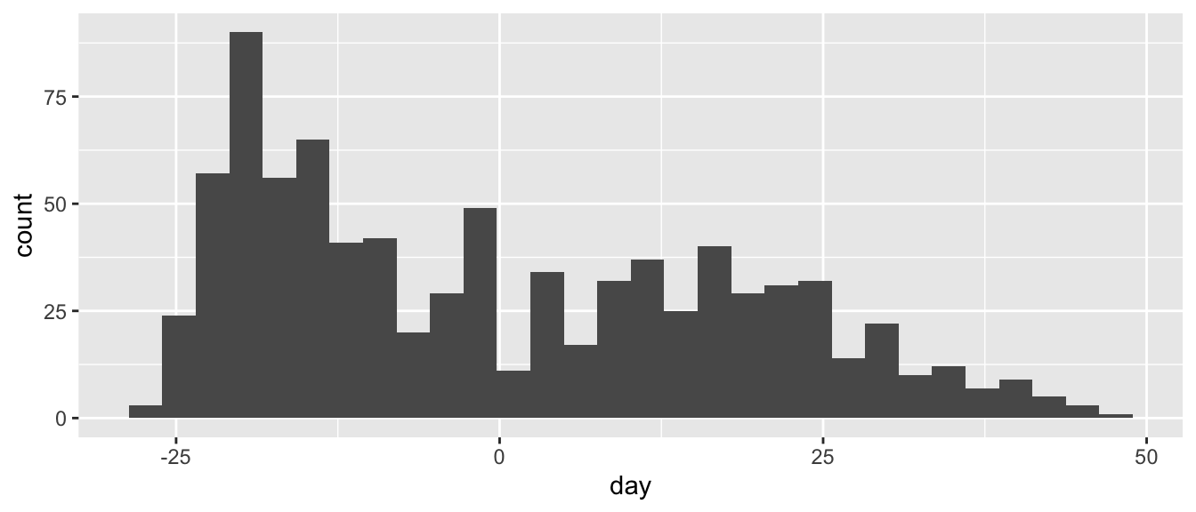
- Plot how the distribution of nest initiation dates over time varies with parasitization status.
ggplot(d, aes(x = day, fill = parasitized)) +
  geom_histogram(position = "identity", alpha = 0.5)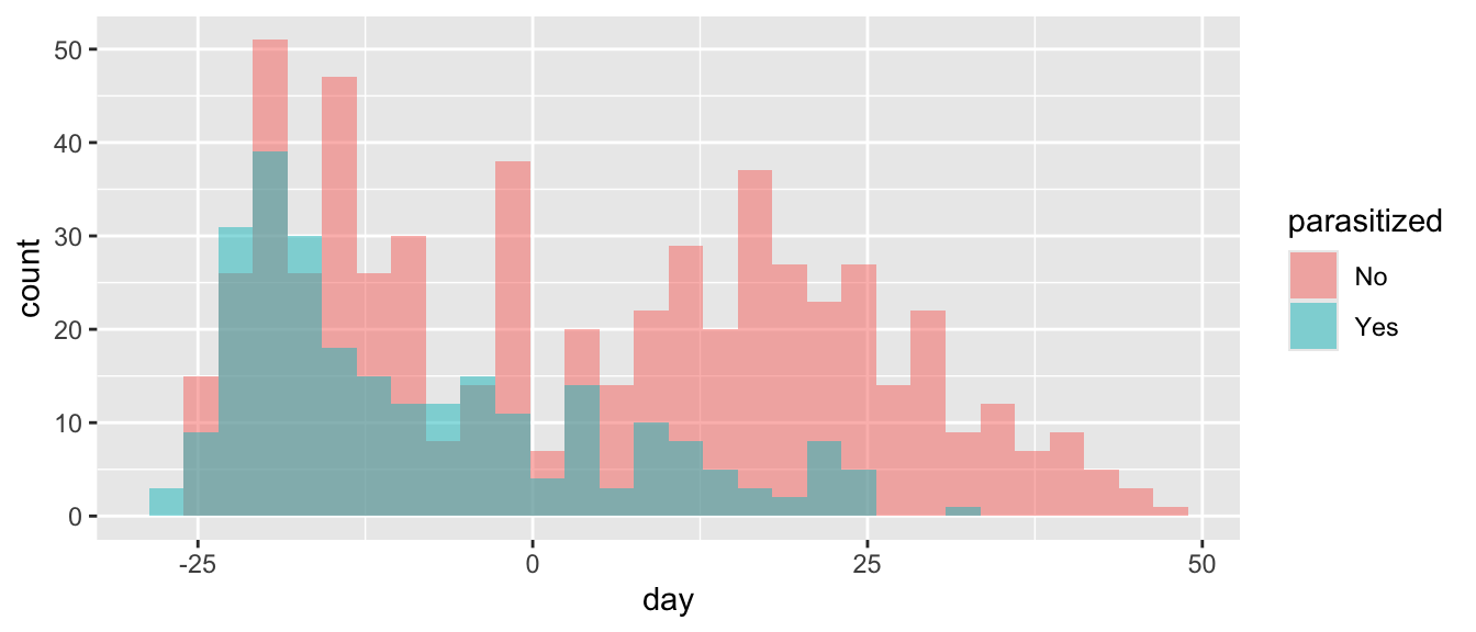
- Plot nest survival (0 or 1) in relation to date of nest initiation and show how this varies with parasitization status. Can you tell if earlier or later initated nests seem more likely to be parasitized?
HINT: When plotting, use geom_jitter() to be able to see individual data points.
ggplot(d |> filter(!is.na(survived)), aes(x = day, y = survived, color = parasitized)) +
  geom_jitter(height = 0.05, alpha = 0.3)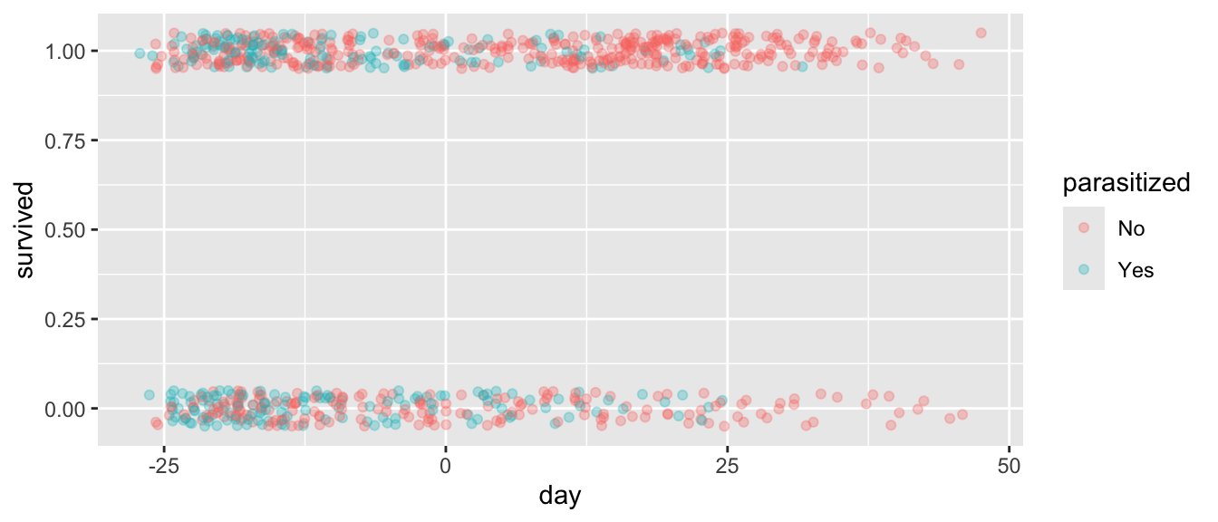
- Plot how the average number of parasitized nests varies across study years.
HINT: This will require computing those averages before or while plotting.
d |>
  select(year, survived) |>
  group_by(year) |>
  filter(!is.na(survived)) |>
  summarize(prop_survived = mean(survived), n = n()) |>
  ggplot(aes(x = year, y = prop_survived, group = 1)) +
  geom_line()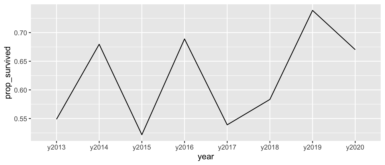
Challenge 2
Run a model to evaluate how the date of nest initiation impacts the probability of parasitism, including year and ID as random effects.
- Given the nature of the data and the response variable, what kind of model would this be?
# Logistic GLMM
m <- glmer(
  parasitized ~
    day +
    (1 | year) +
    (1 | ID),
  data = d,
  family = binomial(link = "logit")
)- Plot the effects of date of nest initiation on probability (not log odds or odds) of the nest being parasitized.
plot_model(m, type = "eff", terms = "day")## You are calculating adjusted predictions on the population-level (i.e.
## `type = "fixed"`) for a *generalized* linear mixed model.
## This may produce biased estimates due to Jensen's inequality. Consider
## setting `bias_correction = TRUE` to correct for this bias.
## See also the documentation of the `bias_correction` argument.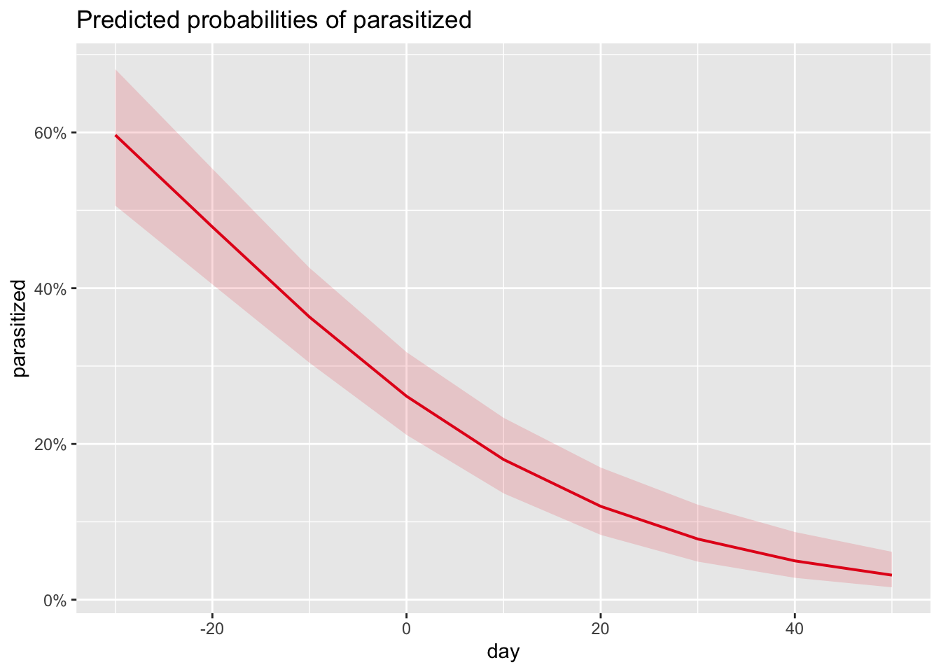
- Based on these model results, does date of nest initiation predict the probability of parasitism? How?
summary(m)## Generalized linear mixed model fit by maximum likelihood (Laplace
## Approximation) [glmerMod]
## Family: binomial ( logit )
## Formula: parasitized ~ day + (1 | year) + (1 | ID)
## Data: d
##
## AIC BIC logLik -2*log(L) df.resid
## 951.7 970.6 -471.8 943.7 843
##
## Scaled residuals:
## Min 1Q Median 3Q Max
## -1.3135 -0.6720 -0.3844 0.9080 2.8867
##
## Random effects:
## Groups Name Variance Std.Dev.
## ID (Intercept) 0.31600 0.5621
## year (Intercept) 0.07421 0.2724
## Number of obs: 847, groups: ID, 468; year, 8
##
## Fixed effects:
## Estimate Std. Error z value Pr(>|z|)
## (Intercept) -1.039290 0.140692 -7.387 1.5e-13 ***
## day -0.047697 0.005769 -8.267 < 2e-16 ***
## ---
## Signif. codes: 0 '***' 0.001 '**' 0.01 '*' 0.05 '.' 0.1 ' ' 1
##
## Correlation of Fixed Effects:
## (Intr)
## day 0.299Challenge 3
Run a model to evaluate how cowbird parasitism affects the number of hooded warbler eggs in the clutch. For this model, use the number of cowbird eggs (NeCB) (not the dichotomous variable parasitized) as one fixed effect and include date of nest initiation as an additional fixed effect, and use year and ID as random effects.
- Given the nature of the data and the response variable, what kind of model would this be?
# Poisson GLMM
m <- glmer(
  NeHW ~
    NeCB +
    day +
    (1 | year) +
    (1 | ID),
  data = d,
  family = poisson(link = "log")
)
## boundary (singular) fit: see help('isSingular')summary(m)## Generalized linear mixed model fit by maximum likelihood (Laplace
## Approximation) [glmerMod]
## Family: poisson ( log )
## Formula: NeHW ~ NeCB + day + (1 | year) + (1 | ID)
## Data: d
##
## AIC BIC logLik -2*log(L) df.resid
## 2711.3 2735.0 -1350.6 2701.3 834
##
## Scaled residuals:
## Min 1Q Median 3Q Max
## -1.63853 -0.24163 0.02492 0.31056 1.37160
##
## Random effects:
## Groups Name Variance Std.Dev.
## ID (Intercept) 0 0
## year (Intercept) 0 0
## Number of obs: 839, groups: ID, 465; year, 8
##
## Fixed effects:
## Estimate Std. Error z value Pr(>|z|)
## (Intercept) 1.188924 0.022773 52.207 < 2e-16 ***
## NeCB -0.267494 0.040001 -6.687 2.28e-11 ***
## day -0.003417 0.001136 -3.008 0.00263 **
## ---
## Signif. codes: 0 '***' 0.001 '**' 0.01 '*' 0.05 '.' 0.1 ' ' 1
##
## Correlation of Fixed Effects:
## (Intr) NeCB
## NeCB -0.489
## day -0.124 0.285
## optimizer (Nelder_Mead) convergence code: 0 (OK)
## boundary (singular) fit: see help('isSingular')NOTE: Running this model as specified above should return a warning about a singular boundary fit. Looking at the random effects table for this model will reveal that neither of the random effects explained any additional variance beyond that explained by the fixed effects, which may indicate model overfitting. For this analysis, the authors of the study from which this dataset comes actually used a GLM instead of a GLMM and included year as an additional fixed effect to still account for inter-annual variation in baseline clutch size. [As in all their models, ID was not included as a random effect.] Try running this alternative model…
# **Poisson GLM**
m <- glm(
  NeHW ~
    NeCB +
    day +
    year,
  data = d,
  family = poisson(link = "log")
)- Plot (separately) the effects of cowbird parasitism and date of initiation on the number of hooded warbler eggs in the clutch.
plot_model(m, type = "eff", terms = "NeCB")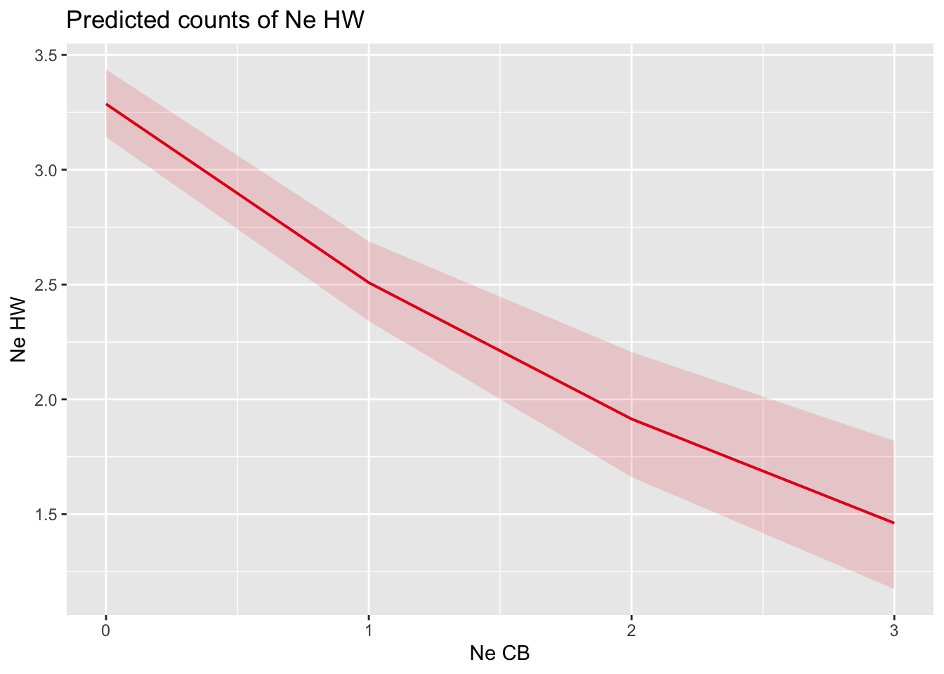
plot_model(m, type = "eff", terms = "day")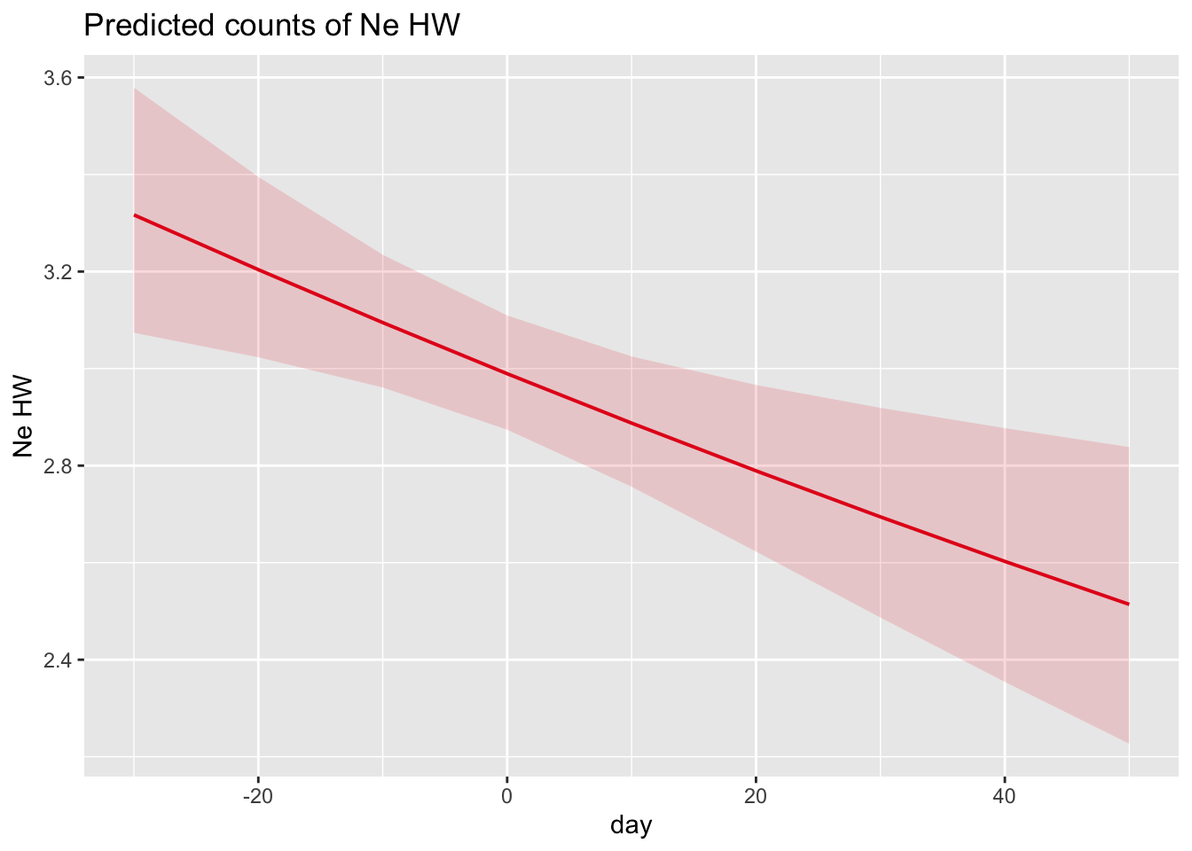
- Is warbler clutch size related to parasitism? Is warbler clutch size related to date of nest initiation?
summary(m)##
## Call:
## glm(formula = NeHW ~ NeCB + day + year, family = poisson(link = "log"),
## data = d)
##
## Coefficients:
## Estimate Std. Error z value Pr(>|z|)
## (Intercept) 1.183809 0.063345 18.688 < 2e-16 ***
## NeCB -0.270168 0.040412 -6.685 2.3e-11 ***
## day -0.003464 0.001148 -3.019 0.00254 **
## yeary2014 0.021927 0.084686 0.259 0.79570
## yeary2015 -0.003269 0.082529 -0.040 0.96840
## yeary2016 -0.012902 0.087896 -0.147 0.88330
## yeary2017 0.002831 0.079932 0.035 0.97175
## yeary2018 -0.008210 0.083430 -0.098 0.92161
## yeary2019 0.017242 0.083329 0.207 0.83608
## yeary2020 0.031198 0.087396 0.357 0.72111
## ---
## Signif. codes: 0 '***' 0.001 '**' 0.01 '*' 0.05 '.' 0.1 ' ' 1
##
## (Dispersion parameter for poisson family taken to be 1)
##
## Null deviance: 295.76 on 838 degrees of freedom
## Residual deviance: 246.66 on 829 degrees of freedom
## (8 observations deleted due to missingness)
## AIC: 2720.8
##
## Number of Fisher Scoring iterations: 4- As a Poisson regression, this model was fit on the log scale. Using the coefficient for NeCB, what is the effect of one additional cowbird egg on the expected number of Hooded Warbler eggs? Express your answer as a multiplicative effect and interpret it in plain language: what happens to expected Hooded Warbler egg count as cowbird eggs increase?
necb <- tidy(m) |>
  filter(term == "NeCB") |>
  pull(estimate)
exp(necb)
## [1] 0.7632516# for every additional cowbird egg, the expected number of Hooded Warbler eggs is multiplied by 0.763, or about a 24% reduction.- What would you expect the number of Hooded Warbler eggs to be for a nest with 2 cowbird eggs compared to a nest with 0 cowbird eggs at the average first lay date (day = 0) and in the earliest year of the study, the reference year (year = y2013)?
int <- tidy(m) |>
  filter(term == "(Intercept)") |>
  pull(estimate)

# 0 cowbird eggs
exp(int + 0 * necb)
## [1] 3.266793# 2 cowbird eggs
exp(int + 2 * necb)## [1] 1.90308# or
newdata <- data.frame(
NeCB = c(0, 2),
day = 0,
year = "y2013"
)
predict(m, newdata = newdata, type = "response")## 1 2
## 3.266793 1.903080Challenge 4
Run a model to examine the probability of nest abandonment in relation to cowbird parasitism. This time use the dichotomous variable parasitized as your fixed factor for cowbird parasitism and, again, include date of initiation as an additional fixed effect and year and ID as random effects.
- Given the nature of the data and the response variable, what kind of model would this be?
# Logistic GLMM
m <- glmer(
  Aban ~
    parasitized +
    day +
    (1 | year) +
    (1 | ID),
  data = d,
  family = binomial(link = "logit")
)
## boundary (singular) fit: see help('isSingular')NOTE: Again, running this model as specified above should return a warning about a singular boundary fit. Run revised models, then, removing each random effect individually and also removing both random effects. You will want to first confirm that your dataset is such that all models are based on the same complete set of data.
d_model <- d |>
  select(Aban, parasitized, day, year, ID) |>
  na.omit()

m <- glmer(
  Aban ~
    parasitized +
    day +
    (1 | year) +
    (1 | ID),
  data = d_model,
  family = binomial(link = "logit")
)

m_no_year <- glmer(
  Aban ~
    parasitized +
    day +
    (1 | ID),
  data = d_model,
  family = binomial(link = "logit")
)

m_no_ID <- glmer(
  Aban ~
    parasitized +
    day +
    (1 | year),
  data = d_model,
  family = binomial(link = "logit")
)

m_no_RE <- glm(
  Aban ~
    parasitized +
    day,
  data = d_model,
  family = binomial(link = "logit")
)- Compare these three additional models to the original one using AICc. See if you can create a nice output table that includes the model name, AIC, AICc, log likelihood, K (df) and deltaAIC values for each model. Recall that AICc = AIC + (2K(K+1))/(n-K-1) and logLik = (AIC = 2K) / (-2). Which is the best model (lowest AICc)?
model_table <-
  AIC(m, m_no_ID, m_no_year, m_no_RE) |>
  rename(K = df) |>
  mutate(
    logLik = (AIC - 2 * K) / (-2),
    AICc = AIC + (2 * K * (K + 1)) / (nrow(d_model) - K - 1),
    deltaAICc = AICc - min(AICc)
  ) |>
  arrange(AICc)
model_table
## K AIC logLik AICc deltaAICc
## m_no_year 4 434.4416 -213.2208 434.4891 0.0000000
## m_no_RE 3 435.0523 -214.5262 435.0808 0.5916682
## m 5 436.4416 -213.2208 436.5130 2.0238378
## m_no_ID 4 437.0220 -214.5110 437.0695 2.5804109- For the best model, plot (first separately, then on the same figure) the marginal effects of cowbird parasitism and date of nest initiation on the probability of nest abandonment. Make sure your Y axis is plotting predicted survival probabilities, not log odds or odds!
HINT: You can do this using either
plot_model()orggpredict().
Remember, the plot_model() function, by default, back-transforms to the probability scale and averages over random effects (here, year).
# predicted P(abandonment) by day averaged over parasitism status
plot_model(m_no_year, type = "eff", terms = "day")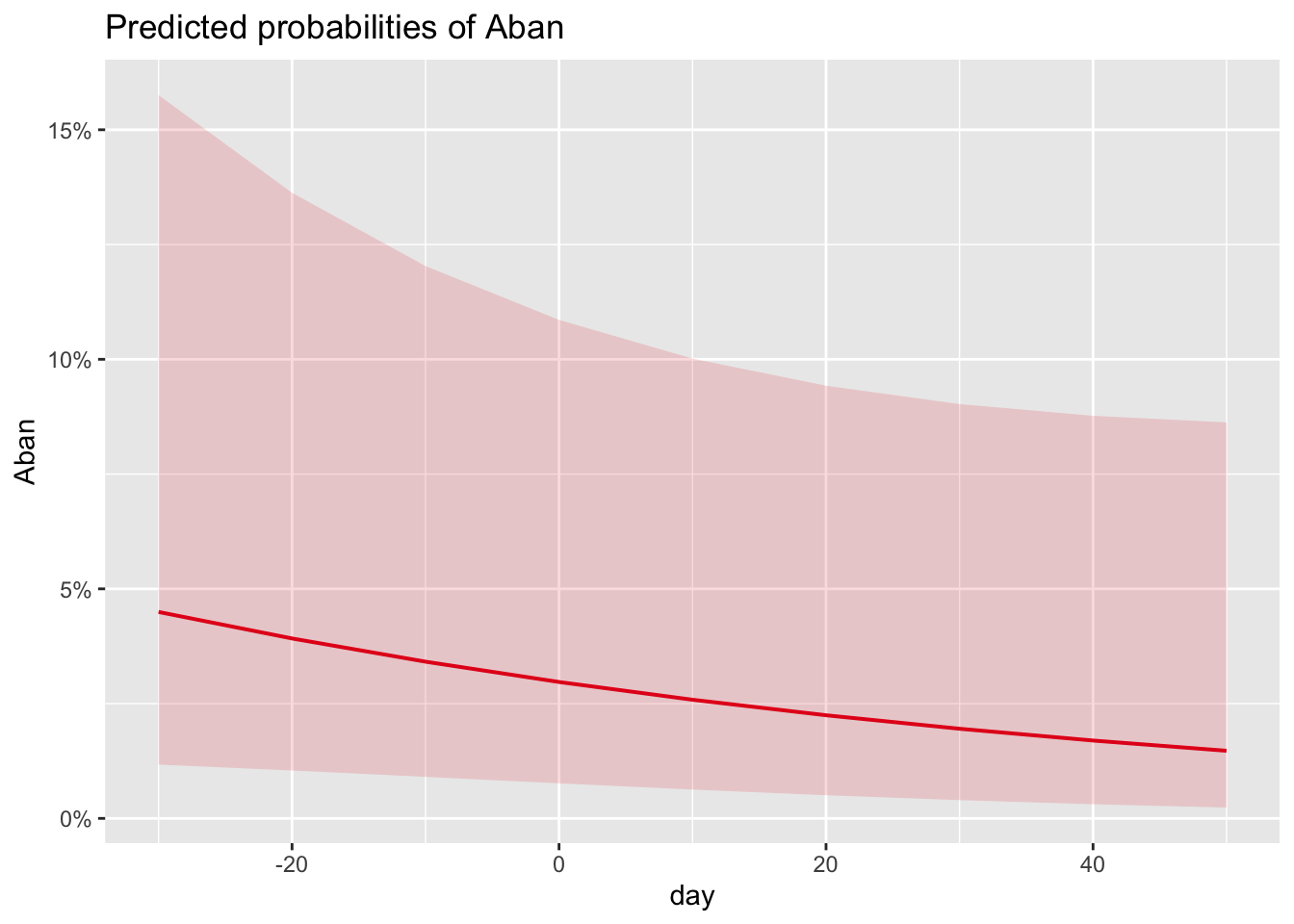
# predicted P(abandonment) by parasitism status, averaged over lay date
plot_model(m_no_year, type = "eff", terms = "parasitized")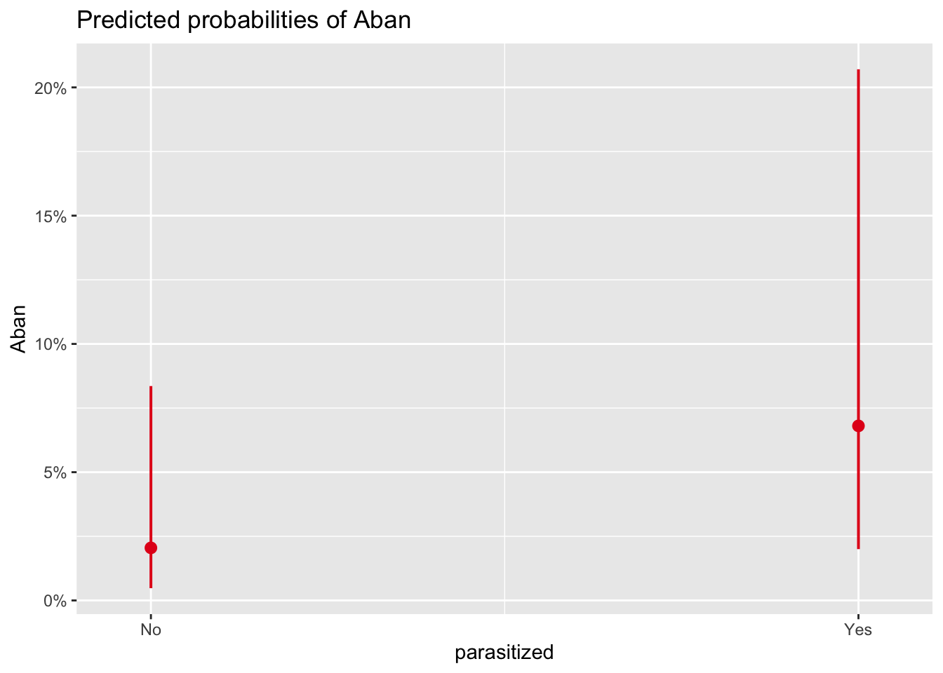
# predicted P(abandonment) across lay dates, separately for parasitized and unparasitized nests
plot_model(m_no_year, type = "eff", terms = c("day", "parasitized"))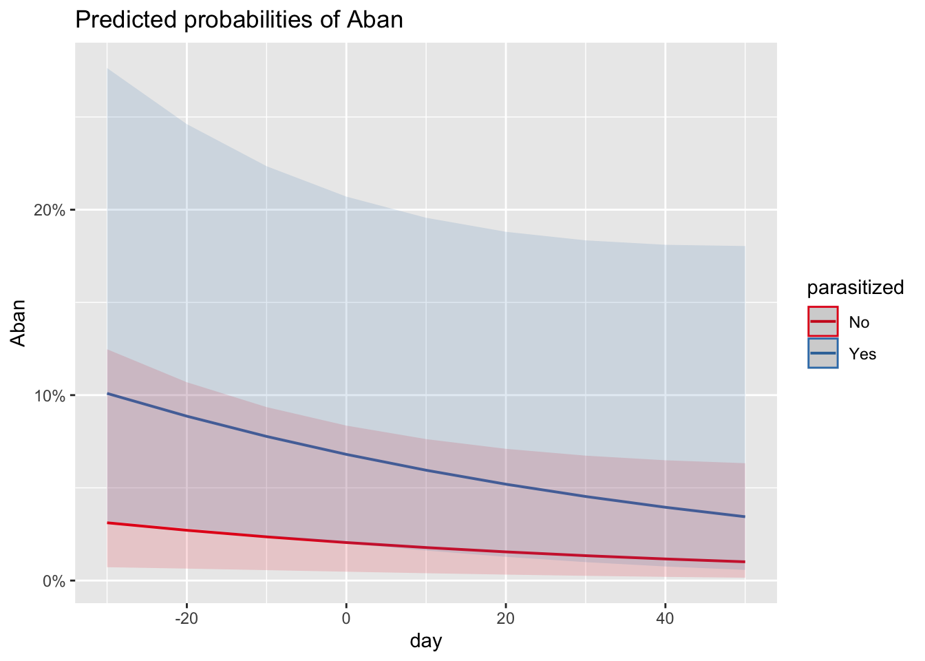
The function ggpredict() from {ggeffects} also back-transforms to the probability scale. For these plots, we use type = "fixed" to get population-level predictions that are not specific to any particular level of our random effect, year. That is, we want marginal predictions that account for the variance associated with the random effects and propagate the uncertainty from the random effects back into the prediction CIs, rather than conditional predictions for a particular level of the random effect. We also use terms = "day [all]" in some of the plots to get smoother looking plots, but we could also just use terms = "day".
# comparable to plot_model(), with marginal effect averaged over other predictor
p1 <- ggpredict(m_no_year, terms = "day [all]", type = "fixed")
plot(p1) + labs(x = "Lay date (centered)", y = "P(abandonment)")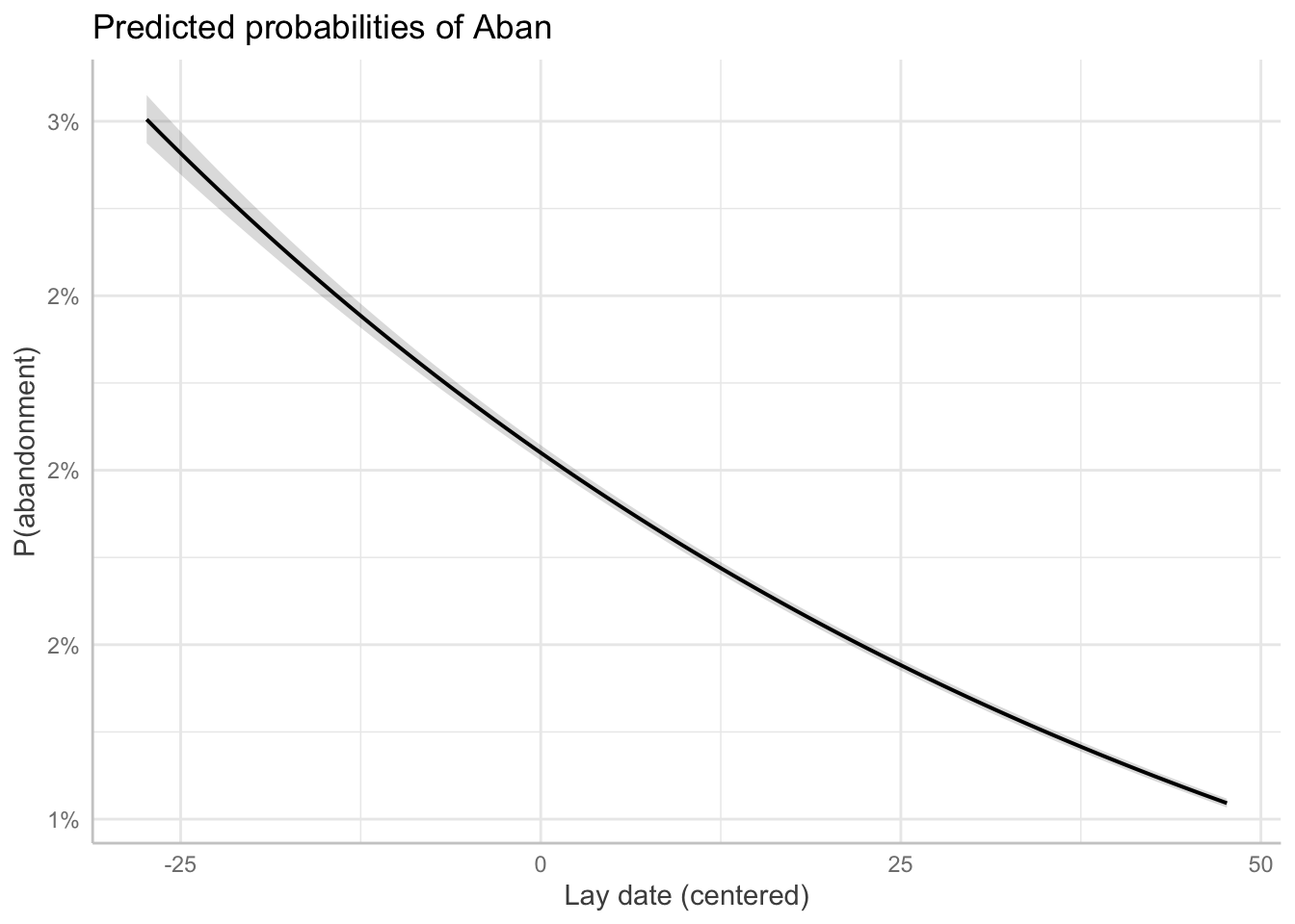
p2 <- ggpredict(m_no_year, terms = "parasitized", type = "fixed")
plot(p2) + labs(x = "Parasitism status", y = "P(abandonment)")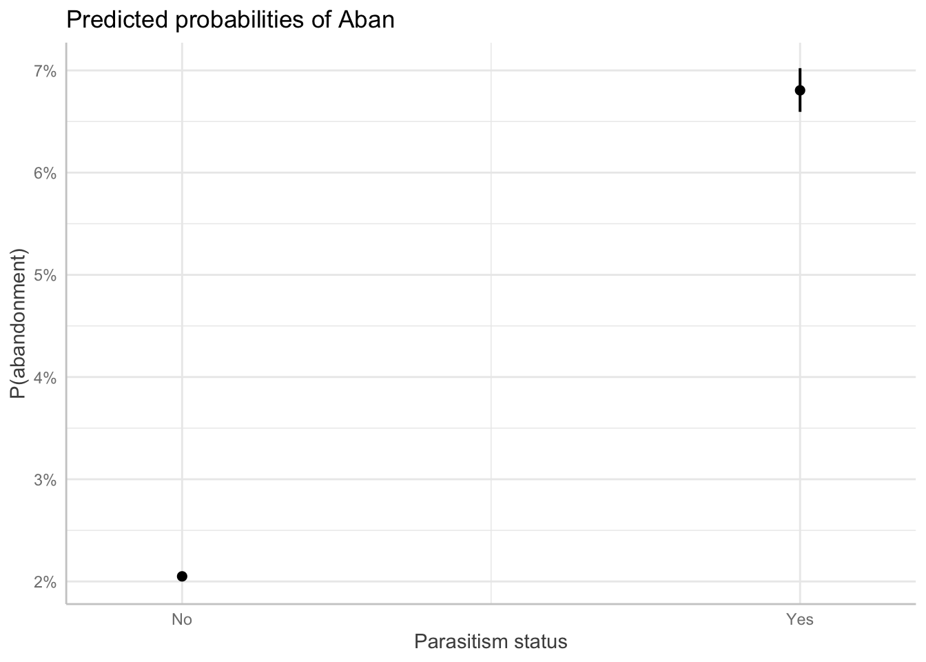
p3 <- ggpredict(m_no_year, terms = c("day [all]", "parasitized"), type = "fixed")

plot(p3) +
  labs(
    x = "Lay date (centered)",
    y = "P(abandonment)",
    color = "Parasitism"
  )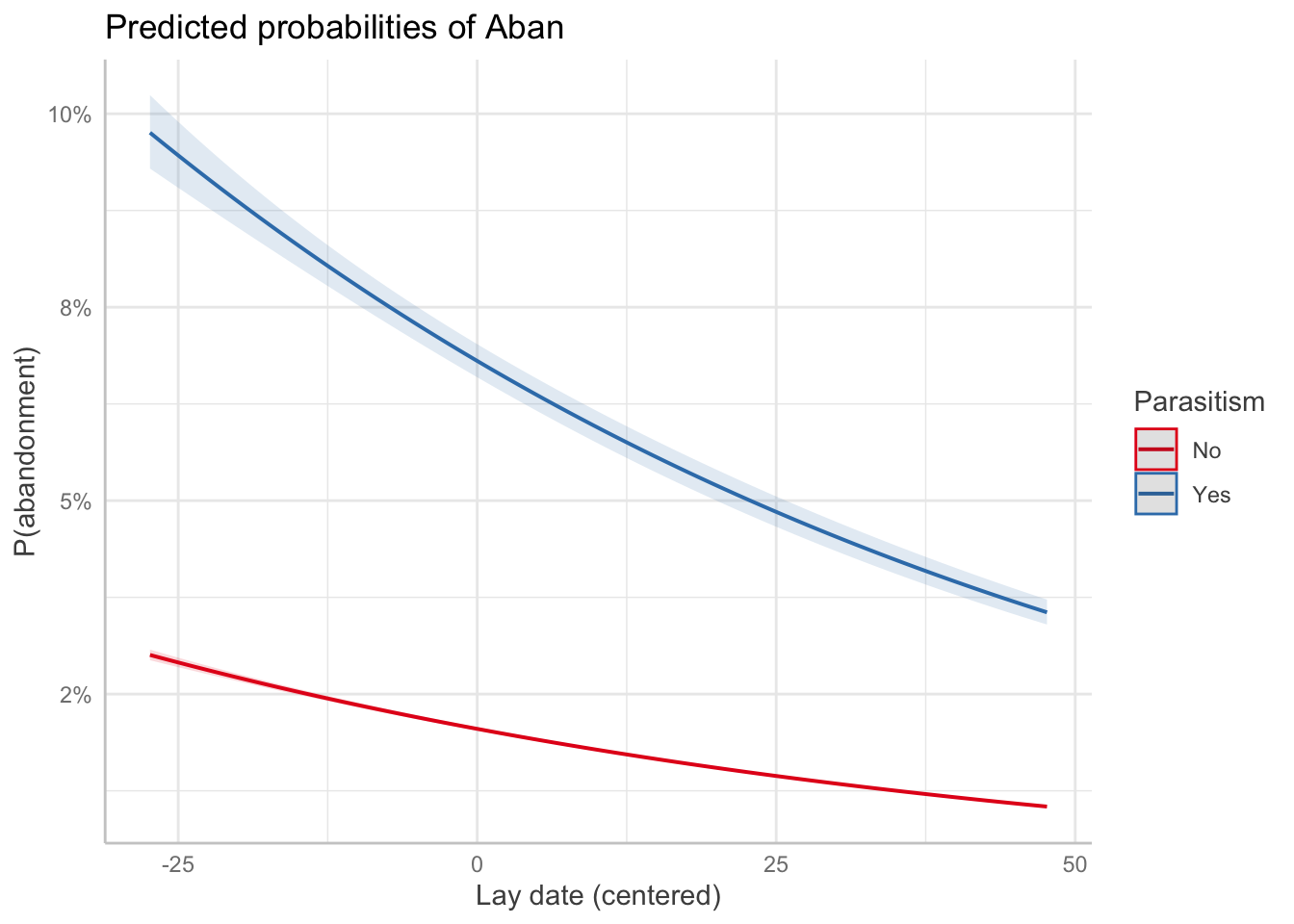
- Under this model, are parasitized nests more likely to be abandoned than unparasitized ones? Is there a relationship between date of nest initiation and probability of nest abandonment?
summary(m_no_year)## Generalized linear mixed model fit by maximum likelihood (Laplace
## Approximation) [glmerMod]
## Family: binomial ( logit )
## Formula: Aban ~ parasitized + day + (1 | ID)
## Data: d_model
##
## AIC BIC logLik -2*log(L) df.resid
## 434.4 453.4 -213.2 426.4 843
##
## Scaled residuals:
## Min 1Q Median 3Q Max
## -0.6478 -0.2450 -0.1474 -0.1206 5.2745
##
## Random effects:
## Groups Name Variance Std.Dev.
## ID (Intercept) 2.293 1.514
## Number of obs: 847, groups: ID, 468
##
## Fixed effects:
## Estimate Std. Error z value Pr(>|z|)
## (Intercept) -3.866599 0.750980 -5.149 2.62e-07 ***
## parasitizedYes 1.249581 0.341288 3.661 0.000251 ***
## day -0.014340 0.009822 -1.460 0.144303
## ---
## Signif. codes: 0 '***' 0.001 '**' 0.01 '*' 0.05 '.' 0.1 ' ' 1
##
## Correlation of Fixed Effects:
## (Intr) prstzY
## parasitzdYs -0.503
## day 0.168 0.224Challenge 5
Run models to examine the probability of nests surviving to hatching in relation to cowbird parasitism. Again, use the dichotomous variable parasitized as your fixed factor for cowbird parasitism and include date of nest initiation as an additional fixed effect and year and ID as random effects. This time, create two models, one excluding and one including an interaction term among the fixed effects.
NOTE: For this analysis, the authors report using a subset of their data limited to 356 nests that were found before the onset of incubation and that were not abandoned. From what I can deduce, they must have run the following to get this subset of data:
d_model <- d |>
filter(Aban == 0, EntAge <= 2, !is.na(survived))- Given the nature of the data and the response variable, what kind of model would this be?
# Logistic GLMM
m <- glmer(
  survived ~
    parasitized +
    day +
    (1 | year) +
    (1 | ID),
  data = d_model,
  family = binomial(link = "logit")
)

m_int <- glmer(
  survived ~
    parasitized *
    day +
    (1 | year) +
    (1 | ID),
  data = d_model,
  family = binomial(link = "logit")
)- Does including the interaction term improve explanatory power over a model with no interaction term?
anova(m, m_int)## Data: d_model
## Models:
## m: survived ~ parasitized + day + (1 | year) + (1 | ID)
## m_int: survived ~ parasitized * day + (1 | year) + (1 | ID)
## npar AIC BIC logLik -2*log(L) Chisq Df Pr(>Chisq)
## m 5 476.06 495.44 -233.03 466.06
## m_int 6 478.05 501.30 -233.03 466.05 0.0106 1 0.9178# fit does not improve with interaction term- Looking at the random effects table in the summary for your model without an interaction term, compare the variance components for year and NestID. What does each tell you about sources of variability in nest survival? Are either random effects contributing meaningfully to the model?
summary(m)## Generalized linear mixed model fit by maximum likelihood (Laplace
## Approximation) [glmerMod]
## Family: binomial ( logit )
## Formula: survived ~ parasitized + day + (1 | year) + (1 | ID)
## Data: d_model
##
## AIC BIC logLik -2*log(L) df.resid
## 476.1 495.4 -233.0 466.1 351
##
## Scaled residuals:
## Min 1Q Median 3Q Max
## -1.8833 -1.1493 0.6357 0.8026 1.0628
##
## Random effects:
## Groups Name Variance Std.Dev.
## ID (Intercept) 0.0311 0.1764
## year (Intercept) 0.0145 0.1204
## Number of obs: 356, groups: ID, 260; year, 8
##
## Fixed effects:
## Estimate Std. Error z value Pr(>|z|)
## (Intercept) 0.612942 0.143878 4.260 2.04e-05 ***
## parasitizedYes -0.381537 0.254776 -1.498 0.1343
## day 0.013412 0.006697 2.003 0.0452 *
## ---
## Signif. codes: 0 '***' 0.001 '**' 0.01 '*' 0.05 '.' 0.1 ' ' 1
##
## Correlation of Fixed Effects:
## (Intr) prstzY
## parasitzdYs -0.499
## day 0.024 0.283# for **year**, there is some between-year variation in baseline survival beyond what is already explained by the fixed effects, meaning some years were slightly better or worse for survival overall regardless of parasitism or date of nest initiation.
# for **ID**, there is also some variation nest survival probability that is attributable to differences between females, beyond what is already explained by the fixed effects.- For this model, what does the intercept coefficient represent? How would you convert this to a probability of nest survival?
# **(Intercept)**: log-odds of survival for nests with average first lay date = 0 and that are unparasitized, where the random effects for **year** and **ID** are at their mean (i.e., an average year, an average female).

int <- tidy(m) |>
  filter(term == "(Intercept)") |>
  pull(estimate)

# convert to response scale
plogis(int)
## [1] 0.6486117# a non-parasitized nest with an average first lay date in an average year has a predicted 65% probability of surviving to hatching- What do the other coefficients represent?
# **parasitizedYes**: the difference in log-odds of survival for parasitized versus non-parasitized nests, holding day constant

parasitizedYes <- tidy(m) |>
  filter(term == "parasitizedYes") |>
  pull(estimate)

# convert to odds scale
exp(parasitizedYes)
## [1] 0.6828112# parasitized nests have 0.68 times the odds of surviving to hatching compared to non-parasitized nests, or about a 32% reduction in odds... however this effect is not significant, so there is not strong evidence that parasitism affects survival to hatching in this model
# **day**: the change in log-odds of nest survival for each one-unit increase in day (i.e., each day later than the average first lay date), holding parasitism constant
day <- tidy(m) |>
filter(term == "day") |>
pull(estimate)
# convert to odds scale
exp(day)## [1] 1.013502# each additional day later than the average first lay date multiplies the odds of surviving by 1.014, or about a 1.4% increase per day... this effect is significant (p < 0.05), suggesting nests initiated later in the season have slightly higher survival odds.
# while a 1.4% increase per day may be statistically detectible, it might be quite small in practical terms- Look at the correlation matrix at the bottom of the summary output of the model. Are the predictors correlated?
# **(Intercept)** and **day** show a correlation of nearly zero, which makes sense and a result of centering day at its mean

# **parasitized** and **day** show a modest positive correlation, meaning parasitized nests tend to be laid slightly later in the season

# this is an interesting biological correlation worth noting... it means parasitism and day are not completely independent predictors, so their individual coefficients should be interpreted holding the other constant (which is what the model does)

# if parasitized nests tend to be initiated later, and later nests survive better, these two effects partially cancel each other out, which may contribute to the non-significant parasitism effect we found
Challenge 6
Run a model to estimate the effects of the presence of a cowbird chick in the nest on the probability of nests surviving from hatching to fledging. Use the dichotomous variable CBHatch as a fixed factor for cowbird parasitism and include date of nest initiation as year as additional fixed effects (following the authors’ analyses, we are excluding random effects).
NOTE: For this analysis, the authors report using a subset of their data limited to 492 nests that were found before hatching that were not abandoned. The column “CBHatch” indicates the presence (1) or absence (0) of a cowbird nestling. From what I can deduce, the authors must have run something like the following to get this subset of data, though this produces a filtered dataset with 497 not 492 rows! The 5-record discrepancy is unresolvable without the authors’ exact cleaning script, which is a useful lesson about reproducibility. The authors should have reported exactly how they got to this subset of 492 records rather than just saying “found before hatching.”
d_model <- d |>
  filter(
    Aban == 0,
    EntAge <= 8,
    FoFAge >= 12,
    !is.na(CBHatch),
    !is.na(day),
    !is.na(survived)
)- Given the nature of the data and the response variable, what kind of model would this be?
# Logistic GLM
# note that *survived* should be numeric (0/1) for binomial GLM, not a factor, so we convert it
d_model <- d_model |>
  mutate(survived = as.numeric(as.character(survived)))

m <- glm(
  survived ~
    CBHatch +
    day +
    year,
  data = d_model,
  family = binomial(link = "logit")
)- Does the presence of a cowbird chick influence the probability of nest survival when the effects of day of nest initiation and study year are taken into account?
summary(m)##
## Call:
## glm(formula = survived ~ CBHatch + day + year, family = binomial(link = "logit"),
## data = d_model)
##
## Coefficients:
## Estimate Std. Error z value Pr(>|z|)
## (Intercept) 9.356e-01 3.233e-01 2.894 0.003803 **
## CBHatch1 1.621e+01 6.695e+02 0.024 0.980677
## day 2.593e-02 7.283e-03 3.560 0.000371 ***
## yeary2014 8.815e-01 4.750e-01 1.856 0.063465 .
## yeary2015 4.871e-01 4.408e-01 1.105 0.269093
## yeary2016 1.232e+00 5.771e-01 2.135 0.032786 *
## yeary2017 4.261e-01 4.435e-01 0.961 0.336630
## yeary2018 7.313e-01 5.067e-01 1.443 0.148946
## yeary2019 1.080e+00 5.206e-01 2.075 0.038027 *
## yeary2020 3.343e-01 4.626e-01 0.723 0.469852
## ---
## Signif. codes: 0 '***' 0.001 '**' 0.01 '*' 0.05 '.' 0.1 ' ' 1
##
## (Dispersion parameter for binomial family taken to be 1)
##
## Null deviance: 454.76 on 496 degrees of freedom
## Residual deviance: 419.25 on 487 degrees of freedom
## AIC: 439.25
##
## Number of Fisher Scoring iterations: 16- Run another model with the number of fledged Hooded Warbler nestlings (NfHW) as the response variable with the same three fixed effects (presence of a cowbird chick, day of nest initiation and study year).
d_model <- d |>
  filter(
    Aban == 0,
    EntAge <= 8,
    FoFAge >= 12,
    !is.na(CBHatch),
    !is.na(day),
    !is.na(NfHW)
  )

m <- glm(
  NfHW ~
    CBHatch +
    day +
    year,
  data = d_model,
  family = poisson(link = "log")
)- Does the presence of a cowbird chick influence the number of successfully fledged Hooded Warbler chicks when the effects of day of nest initiation and study year are taken into account?
summary(m)##
## Call:
## glm(formula = NfHW ~ CBHatch + day + year, family = poisson(link = "log"),
## data = d_model)
##
## Coefficients:
## Estimate Std. Error z value Pr(>|z|)
## (Intercept) 0.757810 0.100526 7.538 4.76e-14 ***
## CBHatch1 -0.868116 0.211091 -4.113 3.91e-05 ***
## day 0.003192 0.001878 1.700 0.08922 .
## yeary2014 -0.311662 0.140761 -2.214 0.02682 *
## yeary2015 -0.105798 0.133333 -0.793 0.42749
## yeary2016 -0.209972 0.149946 -1.400 0.16142
## yeary2017 -0.384265 0.140042 -2.744 0.00607 **
## yeary2018 -0.091316 0.141067 -0.647 0.51742
## yeary2019 -0.191750 0.138947 -1.380 0.16758
## yeary2020 -0.231543 0.141938 -1.631 0.10283
## ---
## Signif. codes: 0 '***' 0.001 '**' 0.01 '*' 0.05 '.' 0.1 ' ' 1
##
## (Dispersion parameter for poisson family taken to be 1)
##
## Null deviance: 915.38 on 493 degrees of freedom
## Residual deviance: 875.45 on 484 degrees of freedom
## AIC: 1759
##
## Number of Fisher Scoring iterations: 5Challenge 7
So far, we have not conducted any diagnostics with the residuals from our regression models. As discussed in Module 24, standard residual plots are misleading for binomial GLMMs. However, the {DHARMa} package is designed for residual diagnostics with mixed models. {DHARMa} uses simulation to create interpretable scaled residuals.
Return to the best model for Challenge 4 about nest abandonment (Aban), which was a GLMM that included two fixed effects (parasitized and day) and one random effect (1 | ID)…
d_model <- d |>
  select(Aban, parasitized, day, year, ID) |>
  na.omit()

m_no_year <- glmer(
  Aban ~
    parasitized +
    day +
    (1 | ID),
  data = d_model,
  family = binomial(link = "logit")
)

summary(m_no_year)
## Generalized linear mixed model fit by maximum likelihood (Laplace
## Approximation) [glmerMod]
## Family: binomial ( logit )
## Formula: Aban ~ parasitized + day + (1 | ID)
## Data: d_model
##
## AIC BIC logLik -2*log(L) df.resid
## 434.4 453.4 -213.2 426.4 843
##
## Scaled residuals:
## Min 1Q Median 3Q Max
## -0.6478 -0.2450 -0.1474 -0.1206 5.2745
##
## Random effects:
## Groups Name Variance Std.Dev.
## ID (Intercept) 2.293 1.514
## Number of obs: 847, groups: ID, 468
##
## Fixed effects:
## Estimate Std. Error z value Pr(>|z|)
## (Intercept) -3.866599 0.750980 -5.149 2.62e-07 ***
## parasitizedYes 1.249581 0.341288 3.661 0.000251 ***
## day -0.014340 0.009822 -1.460 0.144303
## ---
## Signif. codes: 0 '***' 0.001 '**' 0.01 '*' 0.05 '.' 0.1 ' ' 1
##
## Correlation of Fixed Effects:
## (Intr) prstzY
## parasitzdYs -0.503
## day 0.168 0.224- Simulate 1000 residuals under this model.
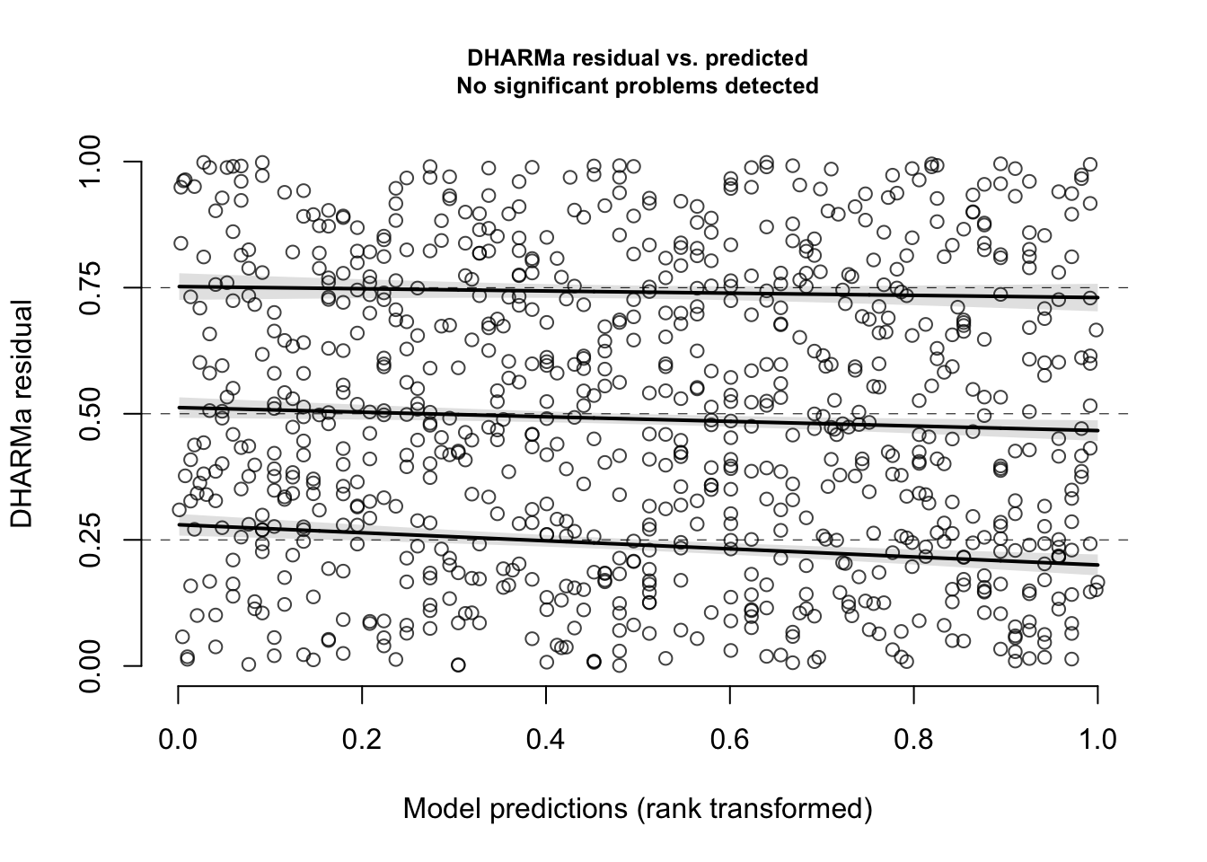
sim <- simulateResiduals(m_no_year, n = 1000)- Examine the residuals for this model. Is there any evidence that the observed residuals deviate from what is expected under the model? Is there any evidence of a relationship between model predictions and residuals? Is there evidence that the residuals are overdispersed, that the model is zero-inflated, or that any observed residuals are clear outliers from what is expected?
plotResiduals(sim)
# tests for uniformity
testUniformity(sim)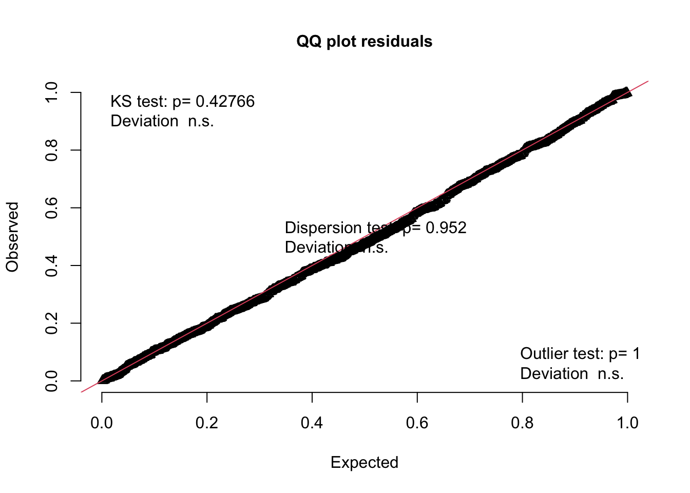
##
##  Asymptotic one-sample Kolmogorov-Smirnov test
##
## data:  simulationOutput$scaledResiduals
## D = 0.030077, p-value = 0.4277
## alternative hypothesis: two-sidedtestCategorical(sim, catPred = d_model$parasitized)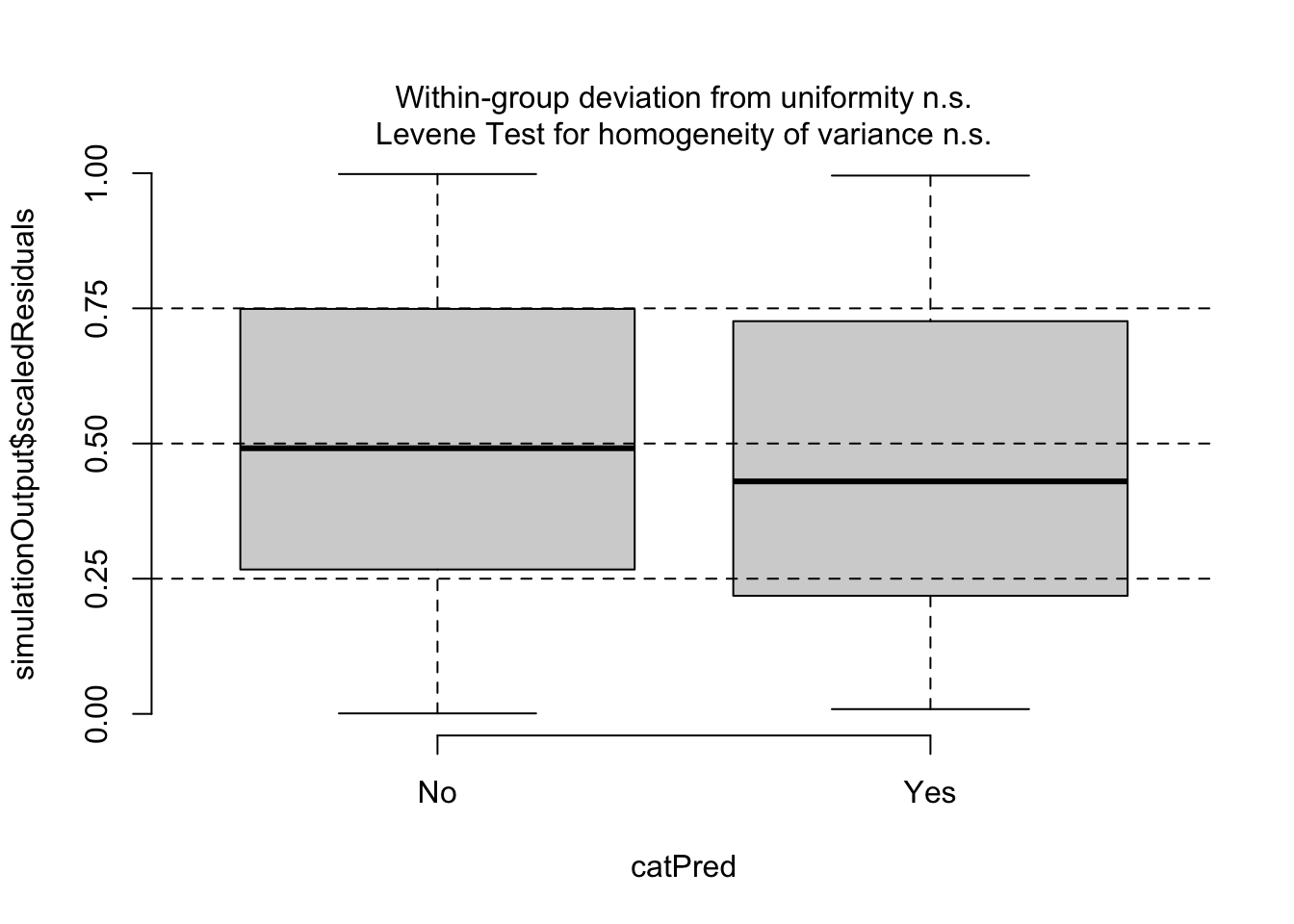
## $uniformity
## $uniformity$details
## catPred: No
##
##  Asymptotic one-sample Kolmogorov-Smirnov test
##
## data:  dd[x, ]
## D = 0.020963, p-value = 0.9581
## alternative hypothesis: two-sided
##
## ------------------------------------------------------------
## catPred: Yes
##
##  Asymptotic one-sample Kolmogorov-Smirnov test
##
## data:  dd[x, ]
## D = 0.076719, p-value = 0.09594
## alternative hypothesis: two-sided
##
##
## $uniformity$p.value
## [1] 0.95805982 0.09593929
##
## $uniformity$p.value.cor
## [1] 0.9580598 0.1918786
##
##
## $homogeneity
## Levene's Test for Homogeneity of Variance (center = median)
##        Df F value Pr(>F)
## group   1  0.7692 0.3807
##       845
# test for overdispersion
testDispersion(sim)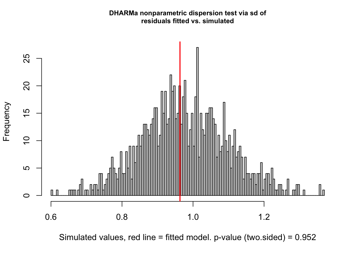
##
##  DHARMa nonparametric dispersion test via sd of residuals fitted vs.
##  simulated
##
## data:  simulationOutput
## dispersion = 0.98708, p-value = 0.952
## alternative hypothesis: two.sided
# test for zero-inflation
testZeroInflation(sim)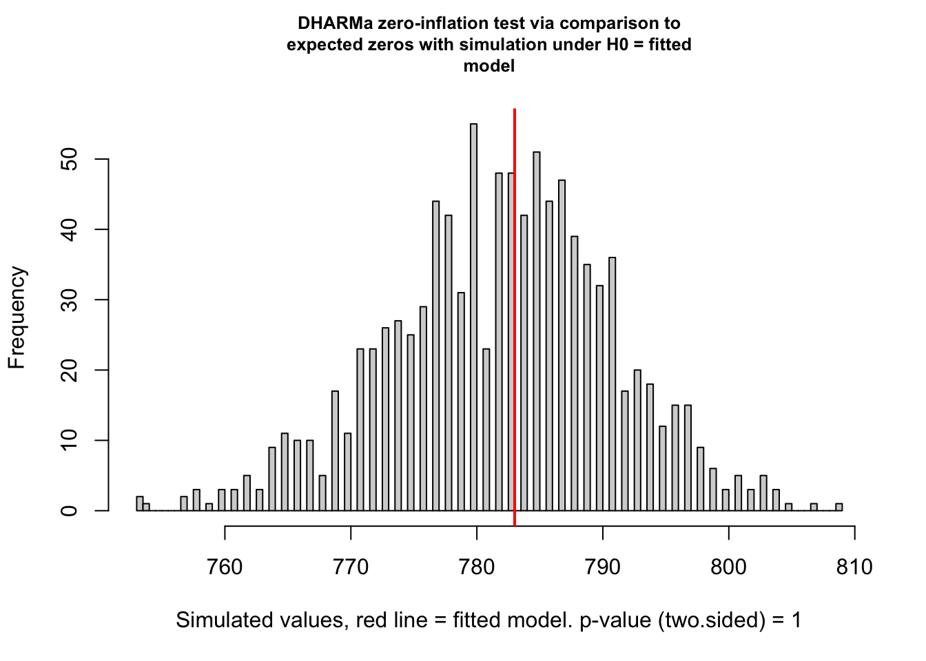
##
##  DHARMa zero-inflation test via comparison to expected zeros with
##  simulation under H0 = fitted model
##
## data:  simulationOutput
## ratioObsSim = 1.0011, p-value = 1
## alternative hypothesis: two.sided
# test for outliers
testOutliers(sim)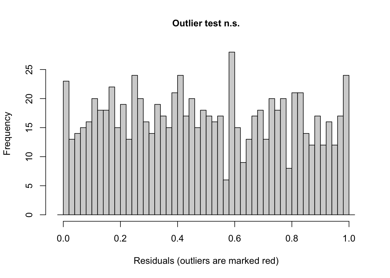
##
##  DHARMa outlier test based on exact binomial test with approximate
##  expectations
##
## data:  sim
## outliers at both margin(s) = 1, observations = 847, p-value = 1
## alternative hypothesis: true probability of success is not equal to 0.001998002
## 95 percent confidence interval:
##  2.989071e-05 6.560366e-03
## sample estimates:
## frequency of outliers (expected: 0.001998001998002 )
##                                          0.001180638
Challenge 8
Again, using the best model from Challenge 4, calculate the variance explained by the fixed effects alone (marginal R²) and by the fixed + random effects (conditional R²).
- How much additional variance in the probability of nest abandonment does including the random effect of ID explain?
r2_nakagawa(m_no_year)## # R2 for Mixed Models
##
## Conditional R2: 0.459
## Marginal R2: 0.081# **marginal R²**: this is the variance explained by the fixed effects alone (i.e., **parasitized** + **day**... these predictors of interest collectively explain about 8% of the variance in nest abandonment
# **conditional R²**: is the variance explained by the fixed effects and the random effect (**ID**)... together they account for 46% of the variance
# note that there is a big difference between these values, thus individual female identity (**ID**) seems to explains a huge amount of variation in the probability of nest abandonment... far more than **parasitism** status or date of nest initiation, i.e., some females are just much more prone to abandoning nests than others, regardless of whether they've been parasitized!Challenge 9
- Extract the individual random effects from the model as a new dataframe (re) using
as.data.frame(ranef(m_no_year))and then plot a histogram of the density distribution of these effects overlaid with a normal distribution.
HINT: The condval column in the re dataframe will contain these individual values.
re <- as.data.frame(ranef(m_no_year))

ggplot(re, aes(x = condval)) +
  geom_histogram(aes(y = after_stat(density))) +
  stat_function(
    fun = dnorm,
    args = list(mean = mean(re$condval), sd = sd(re$condval)),
    colour = "red",
    linewidth = 1
  ) +
  geom_vline(xintercept = 0, linetype = "dashed") +
  labs(
    title = "Distribution of Individual Random Effects",
    subtitle = "Red Curve = Fitted Normal Distribution",
    x = "log-odds deviation from population mean"
  )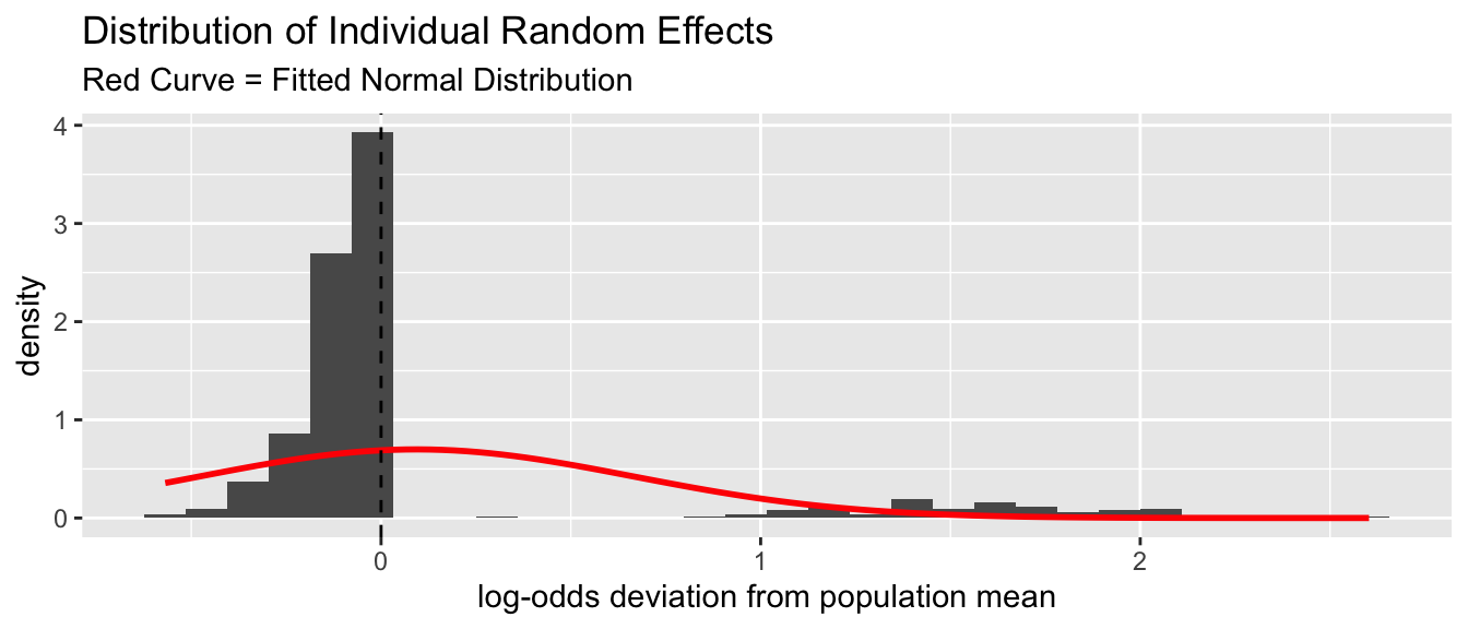
- Do these residuals for the random effect look normal? If not, do they indicate a problem for your regression?
HINT: Use {DHARMa} to simulate residuals from the model and check whether the residuals look okay. This is a more direct test of model fit than looking at the distribution of residuals across individual females.
sim <- simulateResiduals(m_no_year, n = 1000)
plotResiduals(sim)