val <- 45.6
mean <- 50
sd <- 10
(l <- 1 / sqrt(2 * pi * sd^2) * exp((-(val - mean)^2) / (2 * sd^2)))
## [1] 0.03621349This module provides a simple introduction to Maximum Likelihood Estimation and its application in regression analysis.
Maximum Likelihood Estimation (MLE) is a method for estimating population parameters (such as the mean and variance for a normal distribution, the rate parameter (lambda) for a Poisson distribution, the regression coefficients for a linear model) from sample data such that the combined probability (likelihood) of obtaining the observed data is maximized. Here, we first explore the calculation of likelihood values generally and then use MLE to estimate the best parameters for defining from what particular normal distribution a set of data is most likely drawn.
A Probability Density Function (PDF) is a function describing the density of a continuous random variable (a probability mass function, or PMF, is an analogous function for discrete random variables). The function’s value can be calculated at any given point in the sample space (i.e., the range of possible values that the random variable might take) and provides the relative likelihood of obtaining that value on a draw from the given distribution.
The PDF for a normal distribution defined by the parameters \(\mu\) and \(\sigma\) is…
\[f(x | \mu, \sigma) = \frac{1}{\sqrt{2\pi\sigma^2}}e^\frac{-(x-\mu)^2}{2\sigma^2}\]
Where: - \(\mu\) is the mean (or expected value) of the distribution - \(\sigma^2\) is the variance of the distribution. - \(\sigma\) the standard deviation. - \(e\) is the base of the natural logarithm (approximately 2.71828) - \(\pi\) is a mathematical constant (approximately 3.14159)
Solving this function for any value of \(x\) yields the relative likelihood (\(L\)) of drawing that value from the distribution.
As an example, we can calculate the relative likelihood of drawing the number 45.6 out of a normal distribution with a mean (\(\mu\)) of 50 and a standard deviation (\(\sigma\)) of 10…
val <- 45.6
mean <- 50
sd <- 10
(l <- 1 / sqrt(2 * pi * sd^2) * exp((-(val - mean)^2) / (2 * sd^2)))## [1] 0.03621349The dnorm() function returns this relative likelihood directly…
(l <- dnorm(val, mean, sd))## [1] 0.03621349To further explore calculating likelihoods, let’s create and plot a sample of 100 random variables from a normal distribution with a \(\mu\) of 50 and a \(\sigma\) of 10:
set.seed(0) # for reproducibility in rnorm
d <- tibble(val = rnorm(100, mean = 50, sd = 10))
p <- ggplot(d) +
  geom_histogram(aes(x = val, y = after_stat(density)))
p
## `stat_bin()` using `bins = 30`. Pick better value `binwidth`.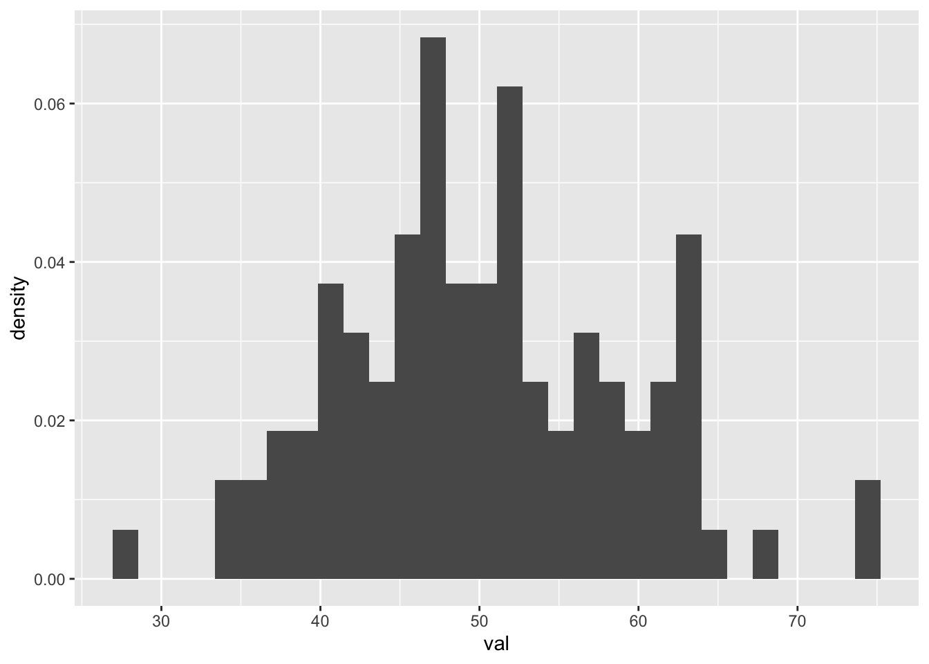
The mean and standard deviation of this sample are pretty are close to the parameters that we pass to the rnorm() function, even though (given the limited size of our sample) the distribution is not smooth…
(mean <- mean(d$val))## [1] 50.22668(sd <- sd(d$val))## [1] 8.826502Now, on top of the histogram of our sample data, let’s plot two different normal distributions, one with the distribution our sample was drawn from (\(\mu\) = 50 and \(\sigma\) = 10, in red) and another with a different \(\mu\) (65) and \(\sigma\) (20).
p <- p +
  stat_function(fun = function(x) dnorm(x, mean = 50, sd = 10), color = "red", linewidth = 1) +
  stat_function(fun = function(x) dnorm(x, mean = 65, sd = 20), color = "blue", linewidth = 1)
p
## `stat_bin()` using `bins = 30`. Pick better value `binwidth`.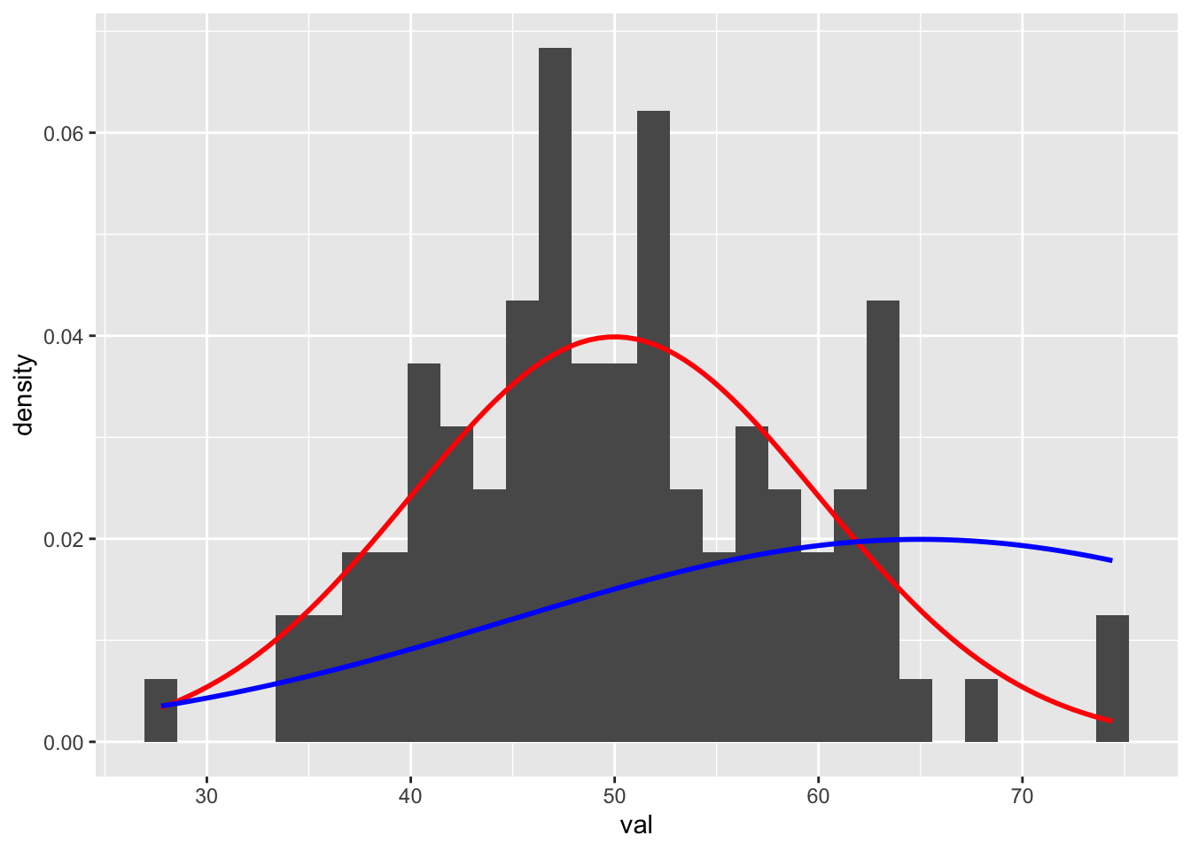
Based on the figure, it should be pretty clear that our observed sample (our set of 100 random draws) is more likely to have been drawn from the former distribution than the latter.
What is the relative likelihood of seeing a value of 41 on a random draw from a normal distribution with \(\mu\) = 50 and \(\sigma\) = 10?
val <- 41
mean <- 50
sd <- 10
# or
(l1 <- dnorm(val, mean, sd))
## [1] 0.02660852What is the relative likelihood of seeing a value of 41 on a random draw from a normal distribution with \(\mu\) = 65 and \(\sigma\) = 20?
val <- 41
mean <- 65
sd <- 10
(l2 <- dnorm(val, mean, sd))
## [1] 0.002239453Note the difference in these two likelihoods, l1 and l2… there is a much higher likelhood of an observation of 41 coming from the first of the two normal distributions we considered. In this case, the likelihood ratio is l1/l2.
l1 / l2## [1] 11.88171We can also calculate the relative likelihood of drawing a particular set of observations from a given distribution as the product of the likelihoods of each observation as the probability of n independent events is simply the product (\(∏\)) of their independent probabilities. An easy way to calculate the product of a set of numbers is by taking the natural log of each number, summing those values, and then exponentiating the sum. For this reason, likelihood calculations are often operationalized in terms of log likelihoods.
For example, the following operations are equivalent…
5 * 8 * 9 * 4## [1] 1440exp(log(5) + log(8) + log(9) + log(4))## [1] 1440exp(sum(log(c(5, 8, 9, 4))))## [1] 1440What is the relative likelihood of drawing the set of three numbers 41, 70, and 10 from a normal distribution with \(\mu\) = 50 and \(\sigma\) = 10?
val <- c(41, 70, 10)
mean <- 65
sd <- 10
(l <- dnorm(val, mean, sd)) # vector of likelihoods of each value
## [1] 2.239453e-03 3.520653e-02 1.076976e-08(l[1] * l[2] * l[3]) # product of likelihoods## [1] 8.491242e-13(ll <- log(l)) # log likelihoods of each value## [1] -6.101524 -3.346524 -18.346524(ll <- sum(ll)) # summed log likelihood## [1] -27.79457(l <- exp(ll)) # convert back to likelihood## [1] 8.491242e-13NOTE: Likelihoods are always going to be zero or greater, but log likelihoods can be negative. A less negative log likelihood is nonetheless more likely than a more negative one.
What are the log likelihood and likelihood of drawing the sample, d, we constructed above from a normal distribution with \(\mu\) = 50 and \(\sigma\) = 10? How do these compare to the log likelihood and likelihood of that same sample being drawn from a normal distribution with \(\mu\) = 65 and \(\sigma\) = 20?
val <- d$val
mean <- 50
sd <- 10
l <- dnorm(val, mean, sd)
ll <- log(l)
ll <- sum(ll)
(l <- exp(ll)) # a very tiny number!
## [1] 2.146356e-157mean <- 65
sd <- 20
l <- dnorm(val, mean, sd)
ll <- log(l)
ll <- sum(ll)
(l <- exp(ll)) # an even tinier number## [1] 8.970731e-187The log likelihood and likelihood are both HIGHER (more likely to have been drawn) from the first distribution.
Now that we have an understanding of how likelihood calculations are done, we can consider the process of maximum likelihood estimation (MLE). MLE allows us to estimate what values of population parameters (e.g., \(\mu\) and \(\sigma\)) are most likely given a dataset and a probability distribution function for the process generating the data (e.g., a Gaussian process).
First, let’s create a function for calculating the negative log likelihood for a set of data under a particular normal distribution. To convert the log likelihood to a negative, we simply multiply it negative 1. The reason we do this is because most optimization algorithms function by searching for parameter values that yield the minimum negative log likelihood rather than the maximum likelihood directly.
verbose_nll <- function(val, mu, sigma, verbose = FALSE) {
  l <- 0 # set initial likelihood to 0 to define variable
  ll <- 0 # set initial log likelihood to 0 to define variable
  for (i in 1:length(val)) {
    l[[i]] <- dnorm(val[[i]], mean = mu, sd = sigma) # likelihoods
    ll[[i]] <- log(l[[i]]) # log likelihoods
    if (verbose == TRUE) {
      message(paste0(
        "x=", round(val[[i]], 4),
        " mu=", mu,
        " sigma=", sigma,
        " L=", round(l[[i]], 4),
        " logL=", round(ll[[i]], 4)
      ))
    }
  }
  nll <- -1 * sum(ll)
  return(nll)
}
Testing our function…
# if we include verbose = TRUE as an argument to `verbose_nll()`, the function will print each likelihood and log likelihood value before returning the summed negative log likelihood
val <- d$val
mean <- 50
sd <- 10
verbose_nll(val, mean, sd, verbose = TRUE)
## x=62.6295 mu=50 sigma=10 L=0.018 logL=-4.0191## x=46.7377 mu=50 sigma=10 L=0.0378 logL=-3.2747## x=63.298 mu=50 sigma=10 L=0.0165 logL=-4.1057## x=62.7243 mu=50 sigma=10 L=0.0178 logL=-4.0311## x=54.1464 mu=50 sigma=10 L=0.0366 logL=-3.3075## x=34.6005 mu=50 sigma=10 L=0.0122 logL=-4.4072## x=40.7143 mu=50 sigma=10 L=0.0259 logL=-3.6526## x=47.0528 mu=50 sigma=10 L=0.0382 logL=-3.265## x=49.9423 mu=50 sigma=10 L=0.0399 logL=-3.2215## x=74.0465 mu=50 sigma=10 L=0.0022 logL=-6.1127## x=57.6359 mu=50 sigma=10 L=0.0298 logL=-3.5131## x=42.0099 mu=50 sigma=10 L=0.029 logL=-3.5407## x=38.5234 mu=50 sigma=10 L=0.0206 logL=-3.8801## x=47.1054 mu=50 sigma=10 L=0.0383 logL=-3.2634## x=47.0078 mu=50 sigma=10 L=0.0381 logL=-3.2663## x=45.8849 mu=50 sigma=10 L=0.0367 logL=-3.3062## x=52.5222 mu=50 sigma=10 L=0.0386 logL=-3.2533## x=41.0808 mu=50 sigma=10 L=0.0268 logL=-3.6193## x=54.3568 mu=50 sigma=10 L=0.0363 logL=-3.3164## x=37.6246 mu=50 sigma=10 L=0.0186 logL=-3.9873## x=47.7573 mu=50 sigma=10 L=0.0389 logL=-3.2467## x=53.774 mu=50 sigma=10 L=0.0372 logL=-3.2927## x=51.3334 mu=50 sigma=10 L=0.0395 logL=-3.2304## x=58.0419 mu=50 sigma=10 L=0.0289 logL=-3.5449## x=49.4289 mu=50 sigma=10 L=0.0398 logL=-3.2232## x=55.0361 mu=50 sigma=10 L=0.0351 logL=-3.3483## x=60.8577 mu=50 sigma=10 L=0.0221 logL=-3.811## x=43.0905 mu=50 sigma=10 L=0.0314 logL=-3.4602## x=37.154 mu=50 sigma=10 L=0.0175 logL=-4.0466## x=50.4673 mu=50 sigma=10 L=0.0399 logL=-3.2226## x=47.6429 mu=50 sigma=10 L=0.0388 logL=-3.2493## x=44.5711 mu=50 sigma=10 L=0.0344 logL=-3.3689## x=45.6669 mu=50 sigma=10 L=0.0363 logL=-3.3154## x=43.5053 mu=50 sigma=10 L=0.0323 logL=-3.4324## x=57.2675 mu=50 sigma=10 L=0.0306 logL=-3.4856## x=61.5191 mu=50 sigma=10 L=0.0205 logL=-3.885## x=59.9216 mu=50 sigma=10 L=0.0244 logL=-3.7137## x=45.7049 mu=50 sigma=10 L=0.0364 logL=-3.3138## x=62.383 mu=50 sigma=10 L=0.0185 logL=-3.9882## x=47.2065 mu=50 sigma=10 L=0.0384 logL=-3.2605## x=67.579 mu=50 sigma=10 L=0.0085 logL=-4.7666## x=55.6075 mu=50 sigma=10 L=0.0341 logL=-3.3787## x=45.4722 mu=50 sigma=10 L=0.036 logL=-3.324## x=41.6796 mu=50 sigma=10 L=0.0282 logL=-3.5677## x=38.3343 mu=50 sigma=10 L=0.0202 logL=-3.902## x=39.3441 mu=50 sigma=10 L=0.0226 logL=-3.7893## x=34.3622 mu=50 sigma=10 L=0.0117 logL=-4.4442## x=61.5654 mu=50 sigma=10 L=0.0204 logL=-3.8903## x=58.3205 mu=50 sigma=10 L=0.0282 logL=-3.5677## x=47.7267 mu=50 sigma=10 L=0.0389 logL=-3.2474## x=52.6614 mu=50 sigma=10 L=0.0385 logL=-3.2569## x=46.233 mu=50 sigma=10 L=0.0372 logL=-3.2925## x=74.4136 mu=50 sigma=10 L=0.002 logL=-6.2017## x=42.0466 mu=50 sigma=10 L=0.0291 logL=-3.5378## x=49.4512 mu=50 sigma=10 L=0.0398 logL=-3.223## x=52.5014 mu=50 sigma=10 L=0.0387 logL=-3.2528## x=56.1824 mu=50 sigma=10 L=0.033 logL=-3.4126## x=48.2738 mu=50 sigma=10 L=0.0393 logL=-3.2364## x=27.761 mu=50 sigma=10 L=0.0034 logL=-5.6944## x=37.3639 mu=50 sigma=10 L=0.018 logL=-4.0199## x=53.5873 mu=50 sigma=10 L=0.0374 logL=-3.2859## x=49.8895 mu=50 sigma=10 L=0.0399 logL=-3.2216## x=40.5935 mu=50 sigma=10 L=0.0256 logL=-3.6639## x=48.8417 mu=50 sigma=10 L=0.0396 logL=-3.2282## x=41.8503 mu=50 sigma=10 L=0.0286 logL=-3.5536## x=52.4226 mu=50 sigma=10 L=0.0387 logL=-3.2509## x=35.749 mu=50 sigma=10 L=0.0145 logL=-4.237## x=53.6594 mu=50 sigma=10 L=0.0373 logL=-3.2885## x=52.4841 mu=50 sigma=10 L=0.0387 logL=-3.2524## x=50.6529 mu=50 sigma=10 L=0.0398 logL=-3.2237## x=50.1916 mu=50 sigma=10 L=0.0399 logL=-3.2217## x=52.5734 mu=50 sigma=10 L=0.0386 logL=-3.2546## x=43.5099 mu=50 sigma=10 L=0.0323 logL=-3.4321## x=48.8083 mu=50 sigma=10 L=0.0396 logL=-3.2286## x=56.6414 mu=50 sigma=10 L=0.032 logL=-3.4421## x=61.0097 mu=50 sigma=10 L=0.0218 logL=-3.8276## x=51.4377 mu=50 sigma=10 L=0.0395 logL=-3.2319## x=48.8225 mu=50 sigma=10 L=0.0396 logL=-3.2285## x=40.8793 mu=50 sigma=10 L=0.0263 logL=-3.6375## x=35.6241 mu=50 sigma=10 L=0.0142 logL=-4.2549## x=42.0291 mu=50 sigma=10 L=0.029 logL=-3.5392## x=62.5408 mu=50 sigma=10 L=0.0182 logL=-4.0079## x=57.7214 mu=50 sigma=10 L=0.0296 logL=-3.5196## x=47.8048 mu=50 sigma=10 L=0.0389 logL=-3.2456## x=45.7519 mu=50 sigma=10 L=0.0365 logL=-3.3118## x=45.8102 mu=50 sigma=10 L=0.0365 logL=-3.3093## x=59.9699 mu=50 sigma=10 L=0.0243 logL=-3.7185## x=47.2422 mu=50 sigma=10 L=0.0384 logL=-3.2596## x=62.5602 mu=50 sigma=10 L=0.0181 logL=-4.0103## x=56.4667 mu=50 sigma=10 L=0.0324 logL=-3.4306## x=62.9931 mu=50 sigma=10 L=0.0172 logL=-4.0656## x=41.2674 mu=50 sigma=10 L=0.0272 logL=-3.6028## x=50.0837 mu=50 sigma=10 L=0.0399 logL=-3.2216## x=41.1913 mu=50 sigma=10 L=0.0271 logL=-3.6095## x=55.9626 mu=50 sigma=10 L=0.0334 logL=-3.3993## x=51.1972 mu=50 sigma=10 L=0.0396 logL=-3.2287## x=47.1783 mu=50 sigma=10 L=0.0383 logL=-3.2613## x=64.5599 mu=50 sigma=10 L=0.0138 logL=-4.2815## x=52.2902 mu=50 sigma=10 L=0.0389 logL=-3.2477## x=59.9654 mu=50 sigma=10 L=0.0243 logL=-3.7181## [1] 360.7421mean <- 65
sd <- 20
verbose_nll(val, mean, sd, verbose = TRUE)## x=62.6295 mu=65 sigma=20 L=0.0198 logL=-3.9217## x=46.7377 mu=65 sigma=20 L=0.0131 logL=-4.3316## x=63.298 mu=65 sigma=20 L=0.0199 logL=-3.9183## x=62.7243 mu=65 sigma=20 L=0.0198 logL=-3.9211## x=54.1464 mu=65 sigma=20 L=0.0172 logL=-4.0619## x=34.6005 mu=65 sigma=20 L=0.0063 logL=-5.0698## x=40.7143 mu=65 sigma=20 L=0.0095 logL=-4.6519## x=47.0528 mu=65 sigma=20 L=0.0133 logL=-4.3173## x=49.9423 mu=65 sigma=20 L=0.015 logL=-4.1981## x=74.0465 mu=65 sigma=20 L=0.018 logL=-4.017## x=57.6359 mu=65 sigma=20 L=0.0186 logL=-3.9825## x=42.0099 mu=65 sigma=20 L=0.0103 logL=-4.5754## x=38.5234 mu=65 sigma=20 L=0.0083 logL=-4.7909## x=47.1054 mu=65 sigma=20 L=0.0134 logL=-4.3149## x=47.0078 mu=65 sigma=20 L=0.0133 logL=-4.3193## x=45.8849 mu=65 sigma=20 L=0.0126 logL=-4.3714## x=52.5222 mu=65 sigma=20 L=0.0164 logL=-4.1093## x=41.0808 mu=65 sigma=20 L=0.0098 logL=-4.6298## x=54.3568 mu=65 sigma=20 L=0.0173 logL=-4.0563## x=37.6246 mu=65 sigma=20 L=0.0078 logL=-4.8514## x=47.7573 mu=65 sigma=20 L=0.0138 logL=-4.2863## x=53.774 mu=65 sigma=20 L=0.017 logL=-4.0722## x=51.3334 mu=65 sigma=20 L=0.0158 logL=-4.1481## x=58.0419 mu=65 sigma=20 L=0.0188 logL=-3.9752## x=49.4289 mu=65 sigma=20 L=0.0147 logL=-4.2177## x=55.0361 mu=65 sigma=20 L=0.0176 logL=-4.0388## x=60.8577 mu=65 sigma=20 L=0.0195 logL=-3.9361## x=43.0905 mu=65 sigma=20 L=0.0109 logL=-4.5147## x=37.154 mu=65 sigma=20 L=0.0076 logL=-4.8839## x=50.4673 mu=65 sigma=20 L=0.0153 logL=-4.1787## x=47.6429 mu=65 sigma=20 L=0.0137 logL=-4.2913## x=44.5711 mu=65 sigma=20 L=0.0118 logL=-4.4363## x=45.6669 mu=65 sigma=20 L=0.0125 logL=-4.3819## x=43.5053 mu=65 sigma=20 L=0.0112 logL=-4.4922## x=57.2675 mu=65 sigma=20 L=0.0185 logL=-3.9894## x=61.5191 mu=65 sigma=20 L=0.0196 logL=-3.9298## x=59.9216 mu=65 sigma=20 L=0.0193 logL=-3.9469## x=45.7049 mu=65 sigma=20 L=0.0125 logL=-4.38## x=62.383 mu=65 sigma=20 L=0.0198 logL=-3.9232## x=47.2065 mu=65 sigma=20 L=0.0134 logL=-4.3104## x=67.579 mu=65 sigma=20 L=0.0198 logL=-3.923## x=55.6075 mu=65 sigma=20 L=0.0179 logL=-4.0249## x=45.4722 mu=65 sigma=20 L=0.0124 logL=-4.3913## x=41.6796 mu=65 sigma=20 L=0.0101 logL=-4.5945## x=38.3343 mu=65 sigma=20 L=0.0082 logL=-4.8035## x=39.3441 mu=65 sigma=20 L=0.0088 logL=-4.7375## x=34.3622 mu=65 sigma=20 L=0.0062 logL=-5.088## x=61.5654 mu=65 sigma=20 L=0.0197 logL=-3.9294## x=58.3205 mu=65 sigma=20 L=0.0189 logL=-3.9704## x=47.7267 mu=65 sigma=20 L=0.0137 logL=-4.2876## x=52.6614 mu=65 sigma=20 L=0.0165 logL=-4.105## x=46.233 mu=65 sigma=20 L=0.0128 logL=-4.3549## x=74.4136 mu=65 sigma=20 L=0.0179 logL=-4.0254## x=42.0466 mu=65 sigma=20 L=0.0103 logL=-4.5732## x=49.4512 mu=65 sigma=20 L=0.0147 logL=-4.2169## x=52.5014 mu=65 sigma=20 L=0.0164 logL=-4.1099## x=56.1824 mu=65 sigma=20 L=0.0181 logL=-4.0119## x=48.2738 mu=65 sigma=20 L=0.0141 logL=-4.2644## x=27.761 mu=65 sigma=20 L=0.0035 logL=-5.6481## x=37.3639 mu=65 sigma=20 L=0.0077 logL=-4.8694## x=53.5873 mu=65 sigma=20 L=0.017 logL=-4.0775## x=49.8895 mu=65 sigma=20 L=0.015 logL=-4.2001## x=40.5935 mu=65 sigma=20 L=0.0095 logL=-4.6593## x=48.8417 mu=65 sigma=20 L=0.0144 logL=-4.241## x=41.8503 mu=65 sigma=20 L=0.0102 logL=-4.5846## x=52.4226 mu=65 sigma=20 L=0.0164 logL=-4.1124## x=35.749 mu=65 sigma=20 L=0.0068 logL=-4.9842## x=53.6594 mu=65 sigma=20 L=0.017 logL=-4.0754## x=52.4841 mu=65 sigma=20 L=0.0164 logL=-4.1105## x=50.6529 mu=65 sigma=20 L=0.0154 logL=-4.172## x=50.1916 mu=65 sigma=20 L=0.0152 logL=-4.1888## x=52.5734 mu=65 sigma=20 L=0.0164 logL=-4.1077## x=43.5099 mu=65 sigma=20 L=0.0112 logL=-4.492## x=48.8083 mu=65 sigma=20 L=0.0144 logL=-4.2424## x=56.6414 mu=65 sigma=20 L=0.0183 logL=-4.002## x=61.0097 mu=65 sigma=20 L=0.0196 logL=-3.9346## x=51.4377 mu=65 sigma=20 L=0.0158 logL=-4.1446## x=48.8225 mu=65 sigma=20 L=0.0144 logL=-4.2418## x=40.8793 mu=65 sigma=20 L=0.0096 logL=-4.6419## x=35.6241 mu=65 sigma=20 L=0.0068 logL=-4.9933## x=42.0291 mu=65 sigma=20 L=0.0103 logL=-4.5742## x=62.5408 mu=65 sigma=20 L=0.0198 logL=-3.9222## x=57.7214 mu=65 sigma=20 L=0.0187 logL=-3.9809## x=47.8048 mu=65 sigma=20 L=0.0138 logL=-4.2843## x=45.7519 mu=65 sigma=20 L=0.0126 logL=-4.3778## x=45.8102 mu=65 sigma=20 L=0.0126 logL=-4.375## x=59.9699 mu=65 sigma=20 L=0.0193 logL=-3.9463## x=47.2422 mu=65 sigma=20 L=0.0134 logL=-4.3088## x=62.5602 mu=65 sigma=20 L=0.0198 logL=-3.9221## x=56.4667 mu=65 sigma=20 L=0.0182 logL=-4.0057## x=62.9931 mu=65 sigma=20 L=0.0198 logL=-3.9197## x=41.2674 mu=65 sigma=20 L=0.0099 logL=-4.6187## x=50.0837 mu=65 sigma=20 L=0.0151 logL=-4.1928## x=41.1913 mu=65 sigma=20 L=0.0098 logL=-4.6232## x=55.9626 mu=65 sigma=20 L=0.018 logL=-4.0168## x=51.1972 mu=65 sigma=20 L=0.0157 logL=-4.1528## x=47.1783 mu=65 sigma=20 L=0.0134 logL=-4.3117## x=64.5599 mu=65 sigma=20 L=0.0199 logL=-3.9149## x=52.2902 mu=65 sigma=20 L=0.0163 logL=-4.1166## x=59.9654 mu=65 sigma=20 L=0.0193 logL=-3.9464## [1] 428.3894… we see that negative log likelihood of our data under the first distribution is smaller than under the second, indicating that it is more likely that are data are drawn from the first distribution.
To use maximum likelihood estimation, we need to create a simpler version of this function that does not have the data as argument, but rather only involves the parameter we want to estimate. The function below does this. Note that unlike the function above, this version does not use a loop and has the vector variable val included as the first argument to the dnorm() function. We also include the argument log = TRUE within the dnorm() function to calculate the log likelihood directly, instead of including that as an extra step.
simple_nll <- function(mu, sigma) {
  ll <- sum(dnorm(val, mean = mu, sd = sigma, log = TRUE))
  nll <- -1 * ll
  return(nll)
}
Testing our function, we should get the same results as above…
val <- d$val
mean <- 50
sd <- 10
simple_nll(mean, sd)
## [1] 360.7421val <- d$val
mean <- 65
sd <- 20
simple_nll(mean, sd)## [1] 428.3894So far, we have just used this function to calculate the (negative) log likelihood of our data being generated by a Gaussian (normal) process with specific \(\mu\) and \(\sigma\) parameters… but what we really want to do is estimate values for \(\mu\) and \(\sigma\) that have highest likelihood for generating our data. To do this, we will use the mle2() function from the {bbmle} package. This function takes the following arguments…
mle2() and the optim() function, which it calls, are highly customizable)NOTE: Be aware that to run the function below, we need to have the variable val, a vector of values, specified outside of the function. We previously set val to d, our random sample of 100 draws from a normal distribution with \(\mu\)=50 and \(\sigma\)=10… feel free to play around with alternatives and see how well the MLE process estimates these parameters.
library(bbmle)

mle_norm <- mle2(
  minuslogl = simple_nll,
  start = list(mu = 0, sigma = 1),
  method = "SANN" # simulated annealing method of optimization, one of several options
)
# note that we may sometimes see a warning about NaNs being produced... this is okay!
mle_norm
##
## Call:
## mle2(minuslogl = simple_nll, start = list(mu = 0, sigma = 1),
## method = "SANN")
##
## Coefficients:
## mu sigma
## 50.2349 8.7631
##
## Log-likelihood: -359.17# note the estimates for `mu` and `sigma` are very close to the population level parameters of the normal distribution that our vector `val` was drawn fromAn alternative for MLE is the maxLik() function from the {maxLik} package. To use function, we again first define our own log likelihood function, but this time we do not want a negative log likelihood, so we do not multiply it by minus 1 (i.e., the first argument maxLik() expects is a log likelihood function, not a negative log likelihood function). Our function should also have only one argument… a vector of parameter values… rather than separate arguments for each parameter.
simple_ll <- function(parameters) {
  # `parameters` is a vector of parameter values
  mu <- parameters[1]
  sigma <- parameters[2]
  ll <- sum(dnorm(val, mean = mu, sd = sigma, log = TRUE))
  return(ll)
}

# test...
simple_ll(c(50, 10)) # this should be very close to the log likelihood returned above
## [1] -360.7421# an alternative function
simple_ll <- function(parameters) {
mu <- parameters[1]
sigma <- parameters[2]
N <- length(val)
ll <- -1 * N * log(sqrt(2 * pi)) - N * log(sigma) - 0.5 * sum((val - mu)^2 / sigma^2)
return(ll)
}
# test...
simple_ll(c(50, 10))## [1] -360.7421As for mle2(), for maxLik() we need to specify several arguments:
mle_norm <- maxLik(logLik = simple_ll, start = c(mu = 0, sigma = 1), method = "NM")
summary(mle_norm)
## --------------------------------------------
## Maximum Likelihood estimation
## Nelder-Mead maximization, 85 iterations
## Return code 0: successful convergence
## Log-Likelihood: -359.1675
## 2 free parameters
## Estimates:
## Estimate Std. error t value Pr(> t)
## mu 50.2392 0.8942 56.18 <2e-16 ***
## sigma 8.7952 0.6323 13.91 <2e-16 ***
## ---
## Signif. codes: 0 '***' 0.001 '**' 0.01 '*' 0.05 '.' 0.1 ' ' 1
## --------------------------------------------The results should be very comparable to those generated using mle2().
Now let’s work through an example of using MLE for simple linear regression. Load in our zombie apocalypse survivors dataset…
f <- "https://raw.githubusercontent.com/difiore/ada-datasets/main/zombies.csv"
d <- read_csv(f, col_names = TRUE)
## Rows: 1000 Columns: 10
## ── Column specification ────────────────────────────────────────────────────────
## Delimiter: ","
## chr (4): first_name, last_name, gender, major
## dbl (6): id, height, weight, zombies_killed, years_of_education, age
##
## ℹ Use `spec()` to retrieve the full column specification for this data.
## ℹ Specify the column types or set `show_col_types = FALSE` to quiet this message.# Standard OLS linear regression model with our zombie apocalypse survivor dataset
m <- lm(data = d, height ~ weight)
summary(m)##
## Call:
## lm(formula = height ~ weight, data = d)
##
## Residuals:
## Min 1Q Median 3Q Max
## -7.1519 -1.5206 -0.0535 1.5167 9.4439
##
## Coefficients:
## Estimate Std. Error t value Pr(>|t|)
## (Intercept) 39.565446 0.595815 66.41 <2e-16 ***
## weight 0.195019 0.004107 47.49 <2e-16 ***
## ---
## Signif. codes: 0 '***' 0.001 '**' 0.01 '*' 0.05 '.' 0.1 ' ' 1
##
## Residual standard error: 2.389 on 998 degrees of freedom
## Multiple R-squared: 0.6932, Adjusted R-squared: 0.6929
## F-statistic: 2255 on 1 and 998 DF, p-value: < 2.2e-16# Compare to...
# Likelihood based linear regression with `mle2()`... now we have our own likelihood function that has three instead of two parameters: b0, b1, and sigma, or the standard deviation in (presumably normally distributed!) residuals...
simple_nll <- function(b0, b1, sigma, verbose = TRUE) {
# here, we say how our expectation for how our response variable, y, is calculated based on two parameters
y <- b0 + b1 * d$weight
N <- nrow(d)
# decomposition of log density function into R terms...
ll <- -1 * N * log(sqrt(2 * pi)) - N * log(sigma) - 0.5 * sum((d$height - y)^2 / sigma^2)
nll <- -1 * ll
return(nll)
}
mle_norm <- mle2(
minuslogl = simple_nll,
# `simple_nll()` is our likelihood function
start = list(b0 = 10, b1 = 0, sigma = 1),
method = "Nelder-Mead"
# implements the Nelder-Mead algorithm for likelihood maximization
)
mle_norm##
## Call:
## mle2(minuslogl = simple_nll, start = list(b0 = 10, b1 = 0, sigma = 1),
## method = "Nelder-Mead")
##
## Coefficients:
## b0 b1 sigma
## 39.5429077 0.1951592 2.3746502
##
## Log-likelihood: -2288.65summary(mle_norm)## Maximum likelihood estimation
##
## Call:
## mle2(minuslogl = simple_nll, start = list(b0 = 10, b1 = 0, sigma = 1),
## method = "Nelder-Mead")
##
## Coefficients:
## Estimate Std. Error z value Pr(z)
## b0 39.542908 0.592347 66.756 < 2.2e-16 ***
## b1 0.195159 0.004083 47.798 < 2.2e-16 ***
## sigma 2.374650 0.052716 45.046 < 2.2e-16 ***
## ---
## Signif. codes: 0 '***' 0.001 '**' 0.01 '*' 0.05 '.' 0.1 ' ' 1
##
## -2 log L: 4577.301# Compare to...
# Likelihood based linear regression with `maxLik()`
loglik <- function(parameters) {
b0 <- parameters[1]
b1 <- parameters[2]
sigma <- parameters[3]
N <- nrow(d)
# here, we say how our expectation for how our response variable, y, is calculated based on parameters
y <- b0 + b1 * d$weight
# estimating mean height as a function of weight
# then use this mu in a similar fashion as previously
ll <- -1 * N * log(sqrt(2 * pi)) - N * log(sigma) - 0.5 * sum((d$height - y)^2 / sigma^2)
return(ll)
}
mle_norm <- maxLik(loglik,
start = c(beta0 = 0, beta1 = 0, sigma = 1),
method = "NM"
)
# implements the Nelder-Mead algorithm for likelihood maximization
summary(mle_norm)## --------------------------------------------
## Maximum Likelihood estimation
## Nelder-Mead maximization, 184 iterations
## Return code 0: successful convergence
## Log-Likelihood: -2288.645
## 3 free parameters
## Estimates:
## Estimate Std. error t value Pr(> t)
## beta0 39.680322 0.950924 41.73 <2e-16 ***
## beta1 0.194221 0.006522 29.78 <2e-16 ***
## sigma 2.387501 0.053872 44.32 <2e-16 ***
## ---
## Signif. codes: 0 '***' 0.001 '**' 0.01 '*' 0.05 '.' 0.1 ' ' 1
## --------------------------------------------# results of both of these should be similar!