7 Additional Data Structures in R

7.1 Objectives

The objective of this module is to introduce additional fundamental data structures in R (matrices, arrays, lists, data frames, and the like) and to learn how to extract, filter, and subset data from them.

7.2 Preliminaries

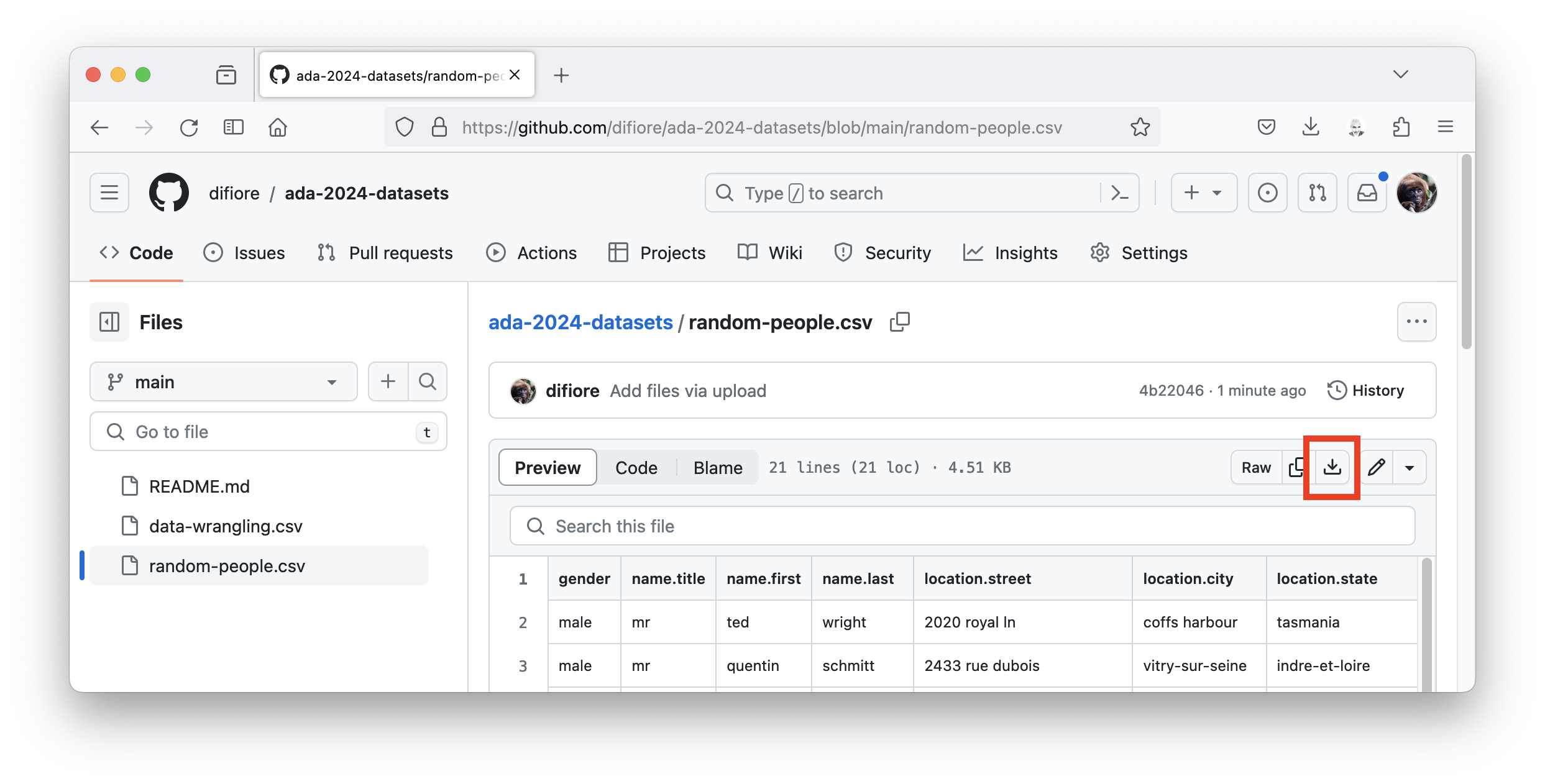
GO TO: https://github.com/difiore/ada-datasets, select the “random-people.csv” file, then press the “Download” button and save the file to your local computer (e.g., on your desktop).

Alternatively, you can press the “Raw” button, highlight, and copy the text to a text editor, and save it. RStudio, as we have seen, has a powerful built-in text editor. There are also a number of other excellent text editors that you download for FREE (e.g., BBEdit for MacOS, Notepad++ for Windows, or Visual Studio Code for either operating system).

Install and load these packages in R: {tidyverse} (which includes {ggplot2}, {dplyr}, {readr}, {tibble}, and {tidyr}, plus others, so they do not need to be installed separately) and {data.table}

7.3 Matrices and Arrays

So far, we have seen several way of creating vectors, which are the most fundamental data structures in R. Today, we will explore and learn how to manipulate other fundamental data structures, including matrices, arrays, lists, and data frames, as well as variants on data frames (e.g., data tables and “tibbles”.)

NOTE: The kind of vectors we have been talking about so far are also sometimes referred to as atomic vectors, and all of the elements of a vector have to have the same data type. We can think of lists (see below) as a different kind of vector, where the elements can have different types, but I prefer to consider lists as a different kind of data structure. Wickham (2019) Advanced R, Second Edition discusses the nuances of various R data structures in more detail.

Matrices and arrays are extensions of the basic vector data structure, and like vectors, all of the elements in an array or matrix have to be of the same atomic type.

We can think of a matrix as a two-dimensional structure consisting of several atomic vectors stored together, but, more accurately, a matrix is essentially a single atomic vector that is split either into multiple columns or multiple rows of the same length. Matrices are useful constructs for performing many mathematical and statistical operations. Again, like 1-dimensional atomic vectors, matrices can only store data of one atomic class (e.g., numerical or character). Matrices are created using the matrix() function.

m <- matrix(
  data = c(1, 2, 3, 4),
  nrow = 2,
  ncol = 2
)
m

##      [,1] [,2]
## [1,]    1    3
## [2,]    2    4

Matrices are typically filled column-wise, with the argument, byrow=, set to FALSE by default (note that FALSE is not in quotation marks). This means that the first column of the matrix will be filled first, the second column second, etc.

m <- matrix(
  data = c(1, 2, 3, 4, 5, 6),
  nrow = 2,
  ncol = 3,
  byrow = FALSE
)
m

##      [,1] [,2] [,3]
## [1,]    1    3    5
## [2,]    2    4    6

This pattern can be changed by specifying the byrow= argument as TRUE.

m <- matrix(
  data = c(1, 2, 3, 4, 5, 6),
  nrow = 2,
  ncol = 3,
  byrow = TRUE
)
m

##      [,1] [,2] [,3]
## [1,]    1    2    3
## [2,]    4    5    6

You can also create matrices by binding vectors of the same length together either row-wise (with the function rbind()) or column-wise (with the function cbind()).

v1 <- c(1, 2, 3, 4)
v2 <- c(6, 7, 8, 9)
m1 <- rbind(v1, v2)
m1

##    [,1] [,2] [,3] [,4]
## v1    1    2    3    4
## v2    6    7    8    9

m2 <- cbind(v1, v2)
m2

##      v1 v2
## [1,]  1  6
## [2,]  2  7
## [3,]  3  8
## [4,]  4  9

Standard metadata about a matrix can be extracted using the class(), dim(), names(), rownames(), colnames() and other commands. The dim() command returns an vector containing the number of rows at index position 1 and the number of columns at index position 2.

class(m1)

## [1] "matrix" "array"

class(m2)

## [1] "matrix" "array"

dim(m1)

## [1] 2 4

dim(m2)

## [1] 4 2

colnames(m1)

## NULL

rownames(m1)

## [1] "v1" "v2"

NOTE: In this example, colnames are not defined for m1 since rbind() was used to create the matrix.

colnames(m2)

## [1] "v1" "v2"

rownames(m2)

## NULL

NOTE: Similarly, in this example, rownames are not defined for m2, since cbind() was used to create the matrix.

As we saw with vectors, the structure (str()) and glimpse (dplyr::glimpse()) commands can be applied to any data structure to provide details about that object. These are incredibly useful functions that you will find yourself using over and over again.

str(m1)

##  num [1:2, 1:4] 1 6 2 7 3 8 4 9
##  - attr(*, "dimnames")=List of 2
##   ..$ : chr [1:2] "v1" "v2"
##   ..$ : NULL

str(m2)

##  num [1:4, 1:2] 1 2 3 4 6 7 8 9
##  - attr(*, "dimnames")=List of 2
##   ..$ : NULL
##   ..$ : chr [1:2] "v1" "v2"

The attributes (attributes()) command can be used to list the attributes of a data structure.

attributes(m1)

## $dim
## [1] 2 4
## 
## $dimnames
## $dimnames[[1]]
## [1] "v1" "v2"
## 
## $dimnames[[2]]
## NULL

attr(m1, which = "dim")

## [1] 2 4

attr(m1, which = "dimnames")[[1]]

## [1] "v1" "v2"

attr(m1, which = "dimnames")[[2]]

## NULL

An array is a more general atomic data structure, of which a vector (with 1 implicit dimension) and a matrix (with 2 defined dimensions) are but examples. Arrays can include additional dimensions, but (like vectors and matrices) they can only include elements that are all of the same atomic data class (e.g., numeric, character). The example below shows the construction of a 3 dimensional array with 5 rows, 6 columns, and 3 “levels”). Visualizing higher and higher dimension arrays, obviously, becomes challenging!

a <- array(data = 1:90, dim = c(5, 6, 3))
a

## , , 1
## 
##      [,1] [,2] [,3] [,4] [,5] [,6]
## [1,]    1    6   11   16   21   26
## [2,]    2    7   12   17   22   27
## [3,]    3    8   13   18   23   28
## [4,]    4    9   14   19   24   29
## [5,]    5   10   15   20   25   30
## 
## , , 2
## 
##      [,1] [,2] [,3] [,4] [,5] [,6]
## [1,]   31   36   41   46   51   56
## [2,]   32   37   42   47   52   57
## [3,]   33   38   43   48   53   58
## [4,]   34   39   44   49   54   59
## [5,]   35   40   45   50   55   60
## 
## , , 3
## 
##      [,1] [,2] [,3] [,4] [,5] [,6]
## [1,]   61   66   71   76   81   86
## [2,]   62   67   72   77   82   87
## [3,]   63   68   73   78   83   88
## [4,]   64   69   74   79   84   89
## [5,]   65   70   75   80   85   90

Subsetting

You can reference or extract select elements from vectors, matrices, and arrays by subsetting them using their index position(s) in what is knows as bracket notation ([ ]). For vectors, you would specify an index value in one dimension. For matrices, you would give the index values in two dimensions. For arrays generally, you would give index values for each dimension in the array.

For example, suppose you have the following vector:

v <- 1:100
v

##   [1]   1   2   3   4   5   6   7   8   9  10  11  12  13  14  15  16  17  18
##  [19]  19  20  21  22  23  24  25  26  27  28  29  30  31  32  33  34  35  36
##  [37]  37  38  39  40  41  42  43  44  45  46  47  48  49  50  51  52  53  54
##  [55]  55  56  57  58  59  60  61  62  63  64  65  66  67  68  69  70  71  72
##  [73]  73  74  75  76  77  78  79  80  81  82  83  84  85  86  87  88  89  90
##  [91]  91  92  93  94  95  96  97  98  99 100

You can select the first 15 elements using bracket notation as follows:

v[1:15]

##  [1]  1  2  3  4  5  6  7  8  9 10 11 12 13 14 15

You can also supply a vector of index values as the argument to [ ] to use for subsetting:

v[c(2, 4, 6, 8, 10)]

## [1]  2  4  6  8 10

Similarly, you can also use a function or a calculation to subset a vector. What does the following return?

v <- 101:200
v[seq(from = 1, to = 100, by = 2)]

##  [1] 101 103 105 107 109 111 113 115 117 119 121 123 125 127 129 131 133 135 137
## [20] 139 141 143 145 147 149 151 153 155 157 159 161 163 165 167 169 171 173 175
## [39] 177 179 181 183 185 187 189 191 193 195 197 199

As an example for a matrix, suppose you have the following:

m <- matrix(data = 1:80, nrow = 8, ncol = 10, byrow = FALSE)
m

##      [,1] [,2] [,3] [,4] [,5] [,6] [,7] [,8] [,9] [,10]
## [1,]    1    9   17   25   33   41   49   57   65    73
## [2,]    2   10   18   26   34   42   50   58   66    74
## [3,]    3   11   19   27   35   43   51   59   67    75
## [4,]    4   12   20   28   36   44   52   60   68    76
## [5,]    5   13   21   29   37   45   53   61   69    77
## [6,]    6   14   22   30   38   46   54   62   70    78
## [7,]    7   15   23   31   39   47   55   63   71    79
## [8,]    8   16   24   32   40   48   56   64   72    80

You can extract the element in row 4, column 5 and assign it to a new variable, x, as follows:

x <- m[4, 5]
x

## [1] 36

You can also extract an entire row or an entire column (or set of rows or set of columns) from a matrix by specifying the desired row or column number(s) and leaving the other value blank.

x <- m[4, ] # extracts 4th row
x

##  [1]  4 12 20 28 36 44 52 60 68 76

CHALLENGE

Given the matrix, m, above, extract the 2nd, 3rd, and 6th columns and assign them to the variable x

Show Code

x <- m[, c(2, 3, 6)]
x

Show Output

##      [,1] [,2] [,3]
## [1,]    9   17   41
## [2,]   10   18   42
## [3,]   11   19   43
## [4,]   12   20   44
## [5,]   13   21   45
## [6,]   14   22   46
## [7,]   15   23   47
## [8,]   16   24   48

Given the matrix, m, above, extract the 6th to 8th row and assign them to the variable x

Show Code

x <- m[6:8, ]
x

Show Output

##      [,1] [,2] [,3] [,4] [,5] [,6] [,7] [,8] [,9] [,10]
## [1,]    6   14   22   30   38   46   54   62   70    78
## [2,]    7   15   23   31   39   47   55   63   71    79
## [3,]    8   16   24   32   40   48   56   64   72    80

Given the matrix, m, above, extract the elements from row 2, column 2 to row 6, column 9 and assign them to the variable x

Show Code

x <- m[2:6, 2:9]
x

Show Output

##      [,1] [,2] [,3] [,4] [,5] [,6] [,7] [,8]
## [1,]   10   18   26   34   42   50   58   66
## [2,]   11   19   27   35   43   51   59   67
## [3,]   12   20   28   36   44   52   60   68
## [4,]   13   21   29   37   45   53   61   69
## [5,]   14   22   30   38   46   54   62   70

Overwriting Elements

You can replace elements in a vector or matrix, or even entire rows or columns, by identifying the elements to be replaced and then assigning them new values.

Starting with the matrix, m, defined above, explore what will be the effects of operations below. Pay careful attention to row and column index values, vector recycling, and automated conversion/recasting among data classes.

m[7, 1] <- 564
m[, 8] <- 2
m[2:5, 4:8] <- 1
m[2:5, 4:8] <- c(20, 19, 18, 17)
m[2:5, 4:8] <- matrix(
  data = c(20:1),
  nrow = 4,
  ncol = 5,
  byrow = TRUE
)
m[, 8] <- c("a", "b")

7.4 Lists and Data Frames

Unlike vectors, matrices, and arrays, two other data structures – lists and data frames – can be used to group together a heterogeneous mix of R structures and objects. A single list, for example, could contain a matrix, vector of character strings, vector of factors, an array, even another list.

Lists are created using the list() function where the elements to add to the list are given as arguments to the function, separated by commas. Type in the following example:

s <- c("this", "is", "a", "vector", "of", "strings")
# this is a vector of character strings
m <- matrix(data = 1:40, nrow = 5, ncol = 8) # this is a matrix
b <- FALSE # this is a boolean variable
l <- list(s, m, b)
l

## [[1]]
## [1] "this"    "is"      "a"       "vector"  "of"      "strings"
## 
## [[2]]
##      [,1] [,2] [,3] [,4] [,5] [,6] [,7] [,8]
## [1,]    1    6   11   16   21   26   31   36
## [2,]    2    7   12   17   22   27   32   37
## [3,]    3    8   13   18   23   28   33   38
## [4,]    4    9   14   19   24   29   34   39
## [5,]    5   10   15   20   25   30   35   40
## 
## [[3]]
## [1] FALSE

Subsetting Lists

You can reference or extract elements from a list similarly to how you would from other data structure, except that you use double brackets ([[ ]]) to reference a single element in the list.

l[[2]]

##      [,1] [,2] [,3] [,4] [,5] [,6] [,7] [,8]
## [1,]    1    6   11   16   21   26   31   36
## [2,]    2    7   12   17   22   27   32   37
## [3,]    3    8   13   18   23   28   33   38
## [4,]    4    9   14   19   24   29   34   39
## [5,]    5   10   15   20   25   30   35   40

An extension of this notation can be used to access elements contained within an element in the list. For example:

l[[2]][2, 6]

## [1] 27

l[[2]][2, ]

## [1]  2  7 12 17 22 27 32 37

l[[2]][, 6]

## [1] 26 27 28 29 30

To reference or extract multiple elements from a list, you would use single bracket ([ ]) notation, which would itself return a list. This is called “list slicing”.

l[2:3]

## [[1]]
##      [,1] [,2] [,3] [,4] [,5] [,6] [,7] [,8]
## [1,]    1    6   11   16   21   26   31   36
## [2,]    2    7   12   17   22   27   32   37
## [3,]    3    8   13   18   23   28   33   38
## [4,]    4    9   14   19   24   29   34   39
## [5,]    5   10   15   20   25   30   35   40
## 
## [[2]]
## [1] FALSE

l[c(1, 3)]

## [[1]]
## [1] "this"    "is"      "a"       "vector"  "of"      "strings"
## 
## [[2]]
## [1] FALSE

Using class() and str() (or dplyr::glimpse()) provides details about the our list and its three elements:

class(l)

## [1] "list"

str(l)

## List of 3
##  $ : chr [1:6] "this" "is" "a" "vector" ...
##  $ : int [1:5, 1:8] 1 2 3 4 5 6 7 8 9 10 ...
##  $ : logi FALSE

dplyr::glimpse(l)

## List of 3
##  $ : chr [1:6] "this" "is" "a" "vector" ...
##  $ : int [1:5, 1:8] 1 2 3 4 5 6 7 8 9 10 ...
##  $ : logi FALSE

You can name the elements in a list using the names() function, which adds a name attribute to each list item.

names(l) <- c("string", "matrix", "logical")
names(l)

## [1] "string"  "matrix"  "logical"

You can also use the name of an item in the list to refer to it using the shortcut $ notation. This is the equivalent of using [[ ]] with either the column number or the name of the column in quotation marks as the argument inside of the double bracket.

# all of the following are equivalent!
l$string

## [1] "this"    "is"      "a"       "vector"  "of"      "strings"

l[[1]]

## [1] "this"    "is"      "a"       "vector"  "of"      "strings"

l[["string"]]

## [1] "this"    "is"      "a"       "vector"  "of"      "strings"

# all of the following are equivalent
l$matrix[3, 5]

## [1] 23

l[[2]][3, 5]

## [1] 23

l[["matrix"]][3, 5]

## [1] 23

The data frame is the perhaps the most useful (and most familiar) data structure that we can operate with in R as it most closely aligns with how we tend to represent tabular data, with rows as cases or observations and columns as variables describing those observations (e.g., a measurement of a particular type). Variables tend to be measured using the same units and thus fall into the same data class and can be thought of as analogous to vectors, so a data frame is essentially a list of atomic vectors that all have the same length.

The data.frame() command can be used to create data frames from scratch.

df <-
  data.frame(
    firstName = c("Rick", "Negan", "Dwight", "Maggie", "Michonne"),
    community = c("Alexandria", "Saviors", "Saviors", "Hiltop", "Alexandria"),
    sex = c("M", "M", "M", "F", "F"),
    age = c(42, 40, 33, 28, 31)
  )
df

##   firstName  community sex age
## 1      Rick Alexandria   M  42
## 2     Negan    Saviors   M  40
## 3    Dwight    Saviors   M  33
## 4    Maggie     Hiltop   F  28
## 5  Michonne Alexandria   F  31

More commonly we read tabular data into R from some external data source (see Module 08, which typically results in the table being represented as a data frame. The following code, for example, will read from the file “random-people.csv” stored in a folder called “data” (a data/ directory) located inside a user’s working directory.

df <-
  read.csv(
    file = "data/random-people.csv",
    sep = ",",
    header = TRUE,
    stringsAsFactors = FALSE
  )
# only print select columns of this data frame
# head() means we will also only print the first several rows
head(df[, c(1, 3, 4, 11, 12)])

##   gender name.first name.last login.password           dob
## 1   male        ted    wright          rolex  11/8/73 1:33
## 2   male    quentin   schmitt         norton  5/24/51 3:16
## 3 female      laura  johansen        stevens 5/22/77 21:03
## 4   male     ismael   herrero         303030   8/1/58 9:13
## 5 female     susana    blanco          aloha 12/18/55 3:21
## 6   male      mason    wilson         topdog  6/23/60 9:19

NOTE: To run the example code above, you may need to replace the string in file = "<string>" with the path to where you stored the file on your local computer.

str(df)

## 'data.frame':    20 obs. of  17 variables:
##  $ gender           : chr  "male" "male" "female" "male" ...
##  $ name.title       : chr  "mr" "mr" "ms" "mr" ...
##  $ name.first       : chr  "ted" "quentin" "laura" "ismael" ...
##  $ name.last        : chr  "wright" "schmitt" "johansen" "herrero" ...
##  $ location.street  : chr  "2020 royal ln" "2433 rue dubois" "2142 elmelunden" "3897 calle del barquillo" ...
##  $ location.city    : chr  "coffs harbour" "vitry-sur-seine" "silkeboeg" "gandia" ...
##  $ location.state   : chr  "tasmania" "indre-et-loire" "hovedstaden" "ceuta" ...
##  $ location.postcode: chr  "4126" "99856" "16264" "61349" ...
##  $ email            : chr  "ted.wright@example.com" "quentin.schmitt@example.com" "laura.johansen@example.com" "ismael.herrero@example.com" ...
##  $ login.username   : chr  "organicleopard402" "bluegoose191" "orangebird528" "heavyswan518" ...
##  $ login.password   : chr  "rolex" "norton" "stevens" "303030" ...
##  $ dob              : chr  "11/8/73 1:33" "5/24/51 3:16" "5/22/77 21:03" "8/1/58 9:13" ...
##  $ date.registered  : chr  "5/5/07 20:26" "4/11/11 7:05" "5/16/14 15:53" "2/17/06 16:53" ...
##  $ phone            : chr  "01-0349-5128" "05-72-65-32-21" "81616775" "974-117-403" ...
##  $ cell             : chr  "0449-989-455" "06-83-24-92-41" "697-993-20" "665-791-673" ...
##  $ picture.large    : chr  "https://randomuser.me/api/portraits/men/48.jpg" "https://randomuser.me/api/portraits/men/53.jpg" "https://randomuser.me/api/portraits/women/70.jpg" "https://randomuser.me/api/portraits/men/79.jpg" ...
##  $ nat              : chr  "AU" "FR" "DK" "ES" ...

dplyr::glimpse(df)

## Rows: 20
## Columns: 17
## $ gender            <chr> "male", "male", "female", "male", "female", "male", …
## $ name.title        <chr> "mr", "mr", "ms", "mr", "ms", "mr", "mr", "miss", "m…
## $ name.first        <chr> "ted", "quentin", "laura", "ismael", "susana", "maso…
## $ name.last         <chr> "wright", "schmitt", "johansen", "herrero", "blanco"…
## $ location.street   <chr> "2020 royal ln", "2433 rue dubois", "2142 elmelunden…
## $ location.city     <chr> "coffs harbour", "vitry-sur-seine", "silkeboeg", "ga…
## $ location.state    <chr> "tasmania", "indre-et-loire", "hovedstaden", "ceuta"…
## $ location.postcode <chr> "4126", "99856", "16264", "61349", "29445", "91479",…
## $ email             <chr> "ted.wright@example.com", "quentin.schmitt@example.c…
## $ login.username    <chr> "organicleopard402", "bluegoose191", "orangebird528"…
## $ login.password    <chr> "rolex", "norton", "stevens", "303030", "aloha", "to…
## $ dob               <chr> "11/8/73 1:33", "5/24/51 3:16", "5/22/77 21:03", "8/…
## $ date.registered   <chr> "5/5/07 20:26", "4/11/11 7:05", "5/16/14 15:53", "2/…
## $ phone             <chr> "01-0349-5128", "05-72-65-32-21", "81616775", "974-1…
## $ cell              <chr> "0449-989-455", "06-83-24-92-41", "697-993-20", "665…
## $ picture.large     <chr> "https://randomuser.me/api/portraits/men/48.jpg", "h…
## $ nat               <chr> "AU", "FR", "DK", "ES", "ES", "NZ", "DE", "US", "TR"…

As for other data structures, you can select and subset data frames using single bracket notation ([ ]). You can also select named columns from a data frame using the $ operator or the equivalent double bracket notation ([[ ]]).

# single bracket notation
df[, 4]

##  [1] "wright"     "schmitt"    "johansen"   "herrero"    "blanco"    
##  [6] "wilson"     "strauio"    "gordon"     "limoncuocu" "perrin"    
## [11] "lopez"      "waisanen"   "brewer"     "brown"      "baettner"  
## [16] "wallace"    "gonzalez"   "neva"       "barnaby"    "moser"

str(df[, 4])

##  chr [1:20] "wright" "schmitt" "johansen" "herrero" "blanco" "wilson" ...

# returns the vector of data stored in column 4

The following are all equivalent…

# using the $ operator with the column name
df$name.last

##  [1] "wright"     "schmitt"    "johansen"   "herrero"    "blanco"    
##  [6] "wilson"     "strauio"    "gordon"     "limoncuocu" "perrin"    
## [11] "lopez"      "waisanen"   "brewer"     "brown"      "baettner"  
## [16] "wallace"    "gonzalez"   "neva"       "barnaby"    "moser"

str(df$name.last)

##  chr [1:20] "wright" "schmitt" "johansen" "herrero" "blanco" "wilson" ...

# returns the vector of data stored in column `name.last`

# using double bracket notation and a column index
df[[4]]

##  [1] "wright"     "schmitt"    "johansen"   "herrero"    "blanco"    
##  [6] "wilson"     "strauio"    "gordon"     "limoncuocu" "perrin"    
## [11] "lopez"      "waisanen"   "brewer"     "brown"      "baettner"  
## [16] "wallace"    "gonzalez"   "neva"       "barnaby"    "moser"

str(df[[4]])

##  chr [1:20] "wright" "schmitt" "johansen" "herrero" "blanco" "wilson" ...

# returns the vector of data stored in column 4

# using double bracket notation with the column name
df[["name.last"]]

##  [1] "wright"     "schmitt"    "johansen"   "herrero"    "blanco"    
##  [6] "wilson"     "strauio"    "gordon"     "limoncuocu" "perrin"    
## [11] "lopez"      "waisanen"   "brewer"     "brown"      "baettner"  
## [16] "wallace"    "gonzalez"   "neva"       "barnaby"    "moser"

str(df[["name.last"]])

##  chr [1:20] "wright" "schmitt" "johansen" "herrero" "blanco" "wilson" ...

# returns the vector of data stored in column `name.last`

Note that the following return data structures that are not quite the same as those returned above. Instead, these return data frames rather than vectors!

# using single bracket notation with a column index and no row index
head(df[4])

##   name.last
## 1    wright
## 2   schmitt
## 3  johansen
## 4   herrero
## 5    blanco
## 6    wilson

str(df[4])

## 'data.frame':    20 obs. of  1 variable:
##  $ name.last: chr  "wright" "schmitt" "johansen" "herrero" ...

# returns a data frame of the data from column 4

# using single bracket notation with a column name
head(df["name.last"])

##   name.last
## 1    wright
## 2   schmitt
## 3  johansen
## 4   herrero
## 5    blanco
## 6    wilson

str(df["name.last"])

## 'data.frame':    20 obs. of  1 variable:
##  $ name.last: chr  "wright" "schmitt" "johansen" "herrero" ...

# returns a data frame of the data from column `name.last`

As with matrixes, you can add rows (additional cases) or columns (additional variables) to a data frame using rbind() and cbind().

df <- cbind(df, id = c(1:20))
df <- cbind(df, school = c("UT", "UT", "A&M", "A&M", "UT", "Rice", "Texas Tech", "UT", "UT", "Texas State", "A&M", "UT", "Rice", "UT", "A&M", "Texas Tech", "A&M", "UT", "Texas State", "A&M"))
head(df)

##   gender name.title name.first name.last          location.street
## 1   male         mr        ted    wright            2020 royal ln
## 2   male         mr    quentin   schmitt          2433 rue dubois
## 3 female         ms      laura  johansen          2142 elmelunden
## 4   male         mr     ismael   herrero 3897 calle del barquillo
## 5 female         ms     susana    blanco  2208 avenida de america
## 6   male         mr      mason    wilson         4576 wilson road
##     location.city location.state location.postcode                       email
## 1   coffs harbour       tasmania              4126      ted.wright@example.com
## 2 vitry-sur-seine indre-et-loire             99856 quentin.schmitt@example.com
## 3       silkeboeg    hovedstaden             16264  laura.johansen@example.com
## 4          gandia          ceuta             61349  ismael.herrero@example.com
## 5        mastoles    extremadura             29445   susana.blanco@example.com
## 6         dunedin       taranaki             91479    mason.wilson@example.com
##      login.username login.password           dob date.registered          phone
## 1 organicleopard402          rolex  11/8/73 1:33    5/5/07 20:26   01-0349-5128
## 2      bluegoose191         norton  5/24/51 3:16    4/11/11 7:05 05-72-65-32-21
## 3     orangebird528        stevens 5/22/77 21:03   5/16/14 15:53       81616775
## 4      heavyswan518         303030   8/1/58 9:13   2/17/06 16:53    974-117-403
## 5    silverkoala701          aloha 12/18/55 3:21   10/3/02 17:55    917-199-202
## 6    organicduck470         topdog  6/23/60 9:19    12/1/08 8:31 (137)-326-5772
##             cell                                    picture.large nat id school
## 1   0449-989-455   https://randomuser.me/api/portraits/men/48.jpg  AU  1     UT
## 2 06-83-24-92-41   https://randomuser.me/api/portraits/men/53.jpg  FR  2     UT
## 3     697-993-20 https://randomuser.me/api/portraits/women/70.jpg  DK  3    A&M
## 4    665-791-673   https://randomuser.me/api/portraits/men/79.jpg  ES  4    A&M
## 5    612-612-929 https://randomuser.me/api/portraits/women/18.jpg  ES  5     UT
## 6 (700)-060-1523   https://randomuser.me/api/portraits/men/60.jpg  NZ  6   Rice

Alternatively, you can extend a data frame by adding a new variable directly using the $ operator, like this:

df$school <- c("UT", "UT", "A&M", "A&M", "UT", "Rice", "Texas Tech", "UT", "UT", "Texas State", "A&M", "UT", "Rice", "UT", "A&M", "Texas Tech", "A&M", "UT", "Texas State", "A&M")
head(df)

##   gender name.title name.first name.last          location.street
## 1   male         mr        ted    wright            2020 royal ln
## 2   male         mr    quentin   schmitt          2433 rue dubois
## 3 female         ms      laura  johansen          2142 elmelunden
## 4   male         mr     ismael   herrero 3897 calle del barquillo
## 5 female         ms     susana    blanco  2208 avenida de america
## 6   male         mr      mason    wilson         4576 wilson road
##     location.city location.state location.postcode                       email
## 1   coffs harbour       tasmania              4126      ted.wright@example.com
## 2 vitry-sur-seine indre-et-loire             99856 quentin.schmitt@example.com
## 3       silkeboeg    hovedstaden             16264  laura.johansen@example.com
## 4          gandia          ceuta             61349  ismael.herrero@example.com
## 5        mastoles    extremadura             29445   susana.blanco@example.com
## 6         dunedin       taranaki             91479    mason.wilson@example.com
##      login.username login.password           dob date.registered          phone
## 1 organicleopard402          rolex  11/8/73 1:33    5/5/07 20:26   01-0349-5128
## 2      bluegoose191         norton  5/24/51 3:16    4/11/11 7:05 05-72-65-32-21
## 3     orangebird528        stevens 5/22/77 21:03   5/16/14 15:53       81616775
## 4      heavyswan518         303030   8/1/58 9:13   2/17/06 16:53    974-117-403
## 5    silverkoala701          aloha 12/18/55 3:21   10/3/02 17:55    917-199-202
## 6    organicduck470         topdog  6/23/60 9:19    12/1/08 8:31 (137)-326-5772
##             cell                                    picture.large nat id school
## 1   0449-989-455   https://randomuser.me/api/portraits/men/48.jpg  AU  1     UT
## 2 06-83-24-92-41   https://randomuser.me/api/portraits/men/53.jpg  FR  2     UT
## 3     697-993-20 https://randomuser.me/api/portraits/women/70.jpg  DK  3    A&M
## 4    665-791-673   https://randomuser.me/api/portraits/men/79.jpg  ES  4    A&M
## 5    612-612-929 https://randomuser.me/api/portraits/women/18.jpg  ES  5     UT
## 6 (700)-060-1523   https://randomuser.me/api/portraits/men/60.jpg  NZ  6   Rice

Using the [[ ]] operator with a new variable name in quotation marks works, too:

df[["school"]] <- c("UT", "UT", "A&M", "A&M", "UT", "Rice", "Texas Tech", "UT", "UT", "Texas State", "A&M", "UT", "Rice", "UT", "A&M", "Texas Tech", "A&M", "UT", "Texas State", "A&M")
head(df)

##   gender name.title name.first name.last          location.street
## 1   male         mr        ted    wright            2020 royal ln
## 2   male         mr    quentin   schmitt          2433 rue dubois
## 3 female         ms      laura  johansen          2142 elmelunden
## 4   male         mr     ismael   herrero 3897 calle del barquillo
## 5 female         ms     susana    blanco  2208 avenida de america
## 6   male         mr      mason    wilson         4576 wilson road
##     location.city location.state location.postcode                       email
## 1   coffs harbour       tasmania              4126      ted.wright@example.com
## 2 vitry-sur-seine indre-et-loire             99856 quentin.schmitt@example.com
## 3       silkeboeg    hovedstaden             16264  laura.johansen@example.com
## 4          gandia          ceuta             61349  ismael.herrero@example.com
## 5        mastoles    extremadura             29445   susana.blanco@example.com
## 6         dunedin       taranaki             91479    mason.wilson@example.com
##      login.username login.password           dob date.registered          phone
## 1 organicleopard402          rolex  11/8/73 1:33    5/5/07 20:26   01-0349-5128
## 2      bluegoose191         norton  5/24/51 3:16    4/11/11 7:05 05-72-65-32-21
## 3     orangebird528        stevens 5/22/77 21:03   5/16/14 15:53       81616775
## 4      heavyswan518         303030   8/1/58 9:13   2/17/06 16:53    974-117-403
## 5    silverkoala701          aloha 12/18/55 3:21   10/3/02 17:55    917-199-202
## 6    organicduck470         topdog  6/23/60 9:19    12/1/08 8:31 (137)-326-5772
##             cell                                    picture.large nat id school
## 1   0449-989-455   https://randomuser.me/api/portraits/men/48.jpg  AU  1     UT
## 2 06-83-24-92-41   https://randomuser.me/api/portraits/men/53.jpg  FR  2     UT
## 3     697-993-20 https://randomuser.me/api/portraits/women/70.jpg  DK  3    A&M
## 4    665-791-673   https://randomuser.me/api/portraits/men/79.jpg  ES  4    A&M
## 5    612-612-929 https://randomuser.me/api/portraits/women/18.jpg  ES  5     UT
## 6 (700)-060-1523   https://randomuser.me/api/portraits/men/60.jpg  NZ  6   Rice

NOTE: In the above examples, cbind() results in school being added as a factor while using the $ operator results in school being added as a character vector. You can see this by using the str() command.

A factor is another atomic data class for R for dealing efficiently with nominal variables, usually character strings. Internally, R assigns integer values to each unique string (e.g., 1 for “female”, 2 for “male”, etc.).

Filtering Rows of a Data Frame

An expression that evaluates to a logical vector also be used to subset data frames. Here, we filter the data frame for only those rows where the variable school is “UT”.

new_df <- df[df$school == "UT", ]
new_df

##    gender name.title name.first  name.last         location.street
## 1    male         mr        ted     wright           2020 royal ln
## 2    male         mr    quentin    schmitt         2433 rue dubois
## 5  female         ms     susana     blanco 2208 avenida de america
## 8  female       miss     kaylee     gordon         5475 camden ave
## 9    male         mr     baraek limoncuocu          2664 baedat cd
## 12   male         mr   valtteri   waisanen          9850 hemeentie
## 14 female       miss   kimberly      brown         8654 manor road
## 18 female         ms       ella       neva          4620 visiokatu
##      location.city location.state location.postcode
## 1    coffs harbour       tasmania              4126
## 2  vitry-sur-seine indre-et-loire             99856
## 5         mastoles    extremadura             29445
## 8            flint         oregon             84509
## 9            siirt          tokat             86146
## 12          halsua  south karelia             58124
## 14          bangor        borders          HI92 8RY
## 18          kerava finland proper             26385
##                              email    login.username login.password
## 1           ted.wright@example.com organicleopard402          rolex
## 2      quentin.schmitt@example.com      bluegoose191         norton
## 5        susana.blanco@example.com    silverkoala701          aloha
## 8        kaylee.gordon@example.com beautifulgoose794       atlantis
## 9  baraek.limoncuoculu@example.com whitebutterfly599         tobias
## 12   valtteri.waisanen@example.com        redswan919       nocturne
## 14      kimberly.brown@example.com  crazyelephant996       nebraska
## 18           ella.neva@example.com  orangegorilla786       f00tball
##               dob date.registered          phone           cell
## 1    11/8/73 1:33    5/5/07 20:26   01-0349-5128   0449-989-455
## 2    5/24/51 3:16    4/11/11 7:05 05-72-65-32-21 06-83-24-92-41
## 5   12/18/55 3:21   10/3/02 17:55    917-199-202    612-612-929
## 8   3/24/48 12:22     5/5/13 8:14 (817)-962-1275 (831)-325-1142
## 9    5/8/92 22:01    9/12/04 0:56 (023)-879-4331 (837)-014-1113
## 12 12/24/80 10:40   9/22/03 20:47     02-227-661  042-153-83-79
## 14    1/9/86 8:54    12/3/11 0:41   017684 80873   0799-553-944
## 18  7/18/91 14:30    3/17/14 7:13     02-351-279  043-436-42-30
##                                       picture.large nat id school
## 1    https://randomuser.me/api/portraits/men/48.jpg  AU  1     UT
## 2    https://randomuser.me/api/portraits/men/53.jpg  FR  2     UT
## 5  https://randomuser.me/api/portraits/women/18.jpg  ES  5     UT
## 8  https://randomuser.me/api/portraits/women/65.jpg  US  8     UT
## 9    https://randomuser.me/api/portraits/men/94.jpg  TR  9     UT
## 12   https://randomuser.me/api/portraits/men/80.jpg  FI 12     UT
## 14 https://randomuser.me/api/portraits/women/49.jpg  GB 14     UT
## 18 https://randomuser.me/api/portraits/women/68.jpg  FI 18     UT

In this case, R evaluates the expression df$school == "UT" and returns a logical vector equal in length to the number of rows in df.

df$school == "UT"

##  [1]  TRUE  TRUE FALSE FALSE  TRUE FALSE FALSE  TRUE  TRUE FALSE FALSE  TRUE
## [13] FALSE  TRUE FALSE FALSE FALSE  TRUE FALSE FALSE

It then subsets the original df based on that vector, returning only rows that evaluate to “TRUE”.

The Boolean operators & (for “AND”) and | (for “OR”) can be used to create more complex filtering criteria. Here, we filter the data frame for only those rows where the variable school is “UT” AND the variable gender is “female”.

new_df <- df[df$school == "UT" & df$gender == "female", ]
new_df

##    gender name.title name.first name.last         location.street location.city
## 5  female         ms     susana    blanco 2208 avenida de america      mastoles
## 8  female       miss     kaylee    gordon         5475 camden ave         flint
## 14 female       miss   kimberly     brown         8654 manor road        bangor
## 18 female         ms       ella      neva          4620 visiokatu        kerava
##    location.state location.postcode                      email
## 5     extremadura             29445  susana.blanco@example.com
## 8          oregon             84509  kaylee.gordon@example.com
## 14        borders          HI92 8RY kimberly.brown@example.com
## 18 finland proper             26385      ella.neva@example.com
##       login.username login.password           dob date.registered
## 5     silverkoala701          aloha 12/18/55 3:21   10/3/02 17:55
## 8  beautifulgoose794       atlantis 3/24/48 12:22     5/5/13 8:14
## 14  crazyelephant996       nebraska   1/9/86 8:54    12/3/11 0:41
## 18  orangegorilla786       f00tball 7/18/91 14:30    3/17/14 7:13
##             phone           cell
## 5     917-199-202    612-612-929
## 8  (817)-962-1275 (831)-325-1142
## 14   017684 80873   0799-553-944
## 18     02-351-279  043-436-42-30
##                                       picture.large nat id school
## 5  https://randomuser.me/api/portraits/women/18.jpg  ES  5     UT
## 8  https://randomuser.me/api/portraits/women/65.jpg  US  8     UT
## 14 https://randomuser.me/api/portraits/women/49.jpg  GB 14     UT
## 18 https://randomuser.me/api/portraits/women/68.jpg  FI 18     UT

Here, we filter the data frame for only rows where either the school is “UT” OR the variable gender is “female”, using the | operator. We also select only the columns gender, name.first, and name.last by passing a vector to the second argument of the [ ] function.

new_df <- df[df$school == "UT" | df$gender == "female", c("gender", "name.first", "name.last")]
new_df

##    gender name.first  name.last
## 1    male        ted     wright
## 2    male    quentin    schmitt
## 3  female      laura   johansen
## 5  female     susana     blanco
## 8  female     kaylee     gordon
## 9    male     baraek limoncuocu
## 12   male   valtteri   waisanen
## 13 female    vanessa     brewer
## 14 female   kimberly      brown
## 15 female     loreen   baettner
## 16 female      becky    wallace
## 18 female       ella       neva

Selecting Columns of a Data Frame

We can also select to only return particular columns when we filter. Here, we return only the columns name.last, name.first, and school.

new_df <- df[df$school == "UT", c("name.last", "name.first", "school")]
new_df

##     name.last name.first school
## 1      wright        ted     UT
## 2     schmitt    quentin     UT
## 5      blanco     susana     UT
## 8      gordon     kaylee     UT
## 9  limoncuocu     baraek     UT
## 12   waisanen   valtteri     UT
## 14      brown   kimberly     UT
## 18       neva       ella     UT

Here, we return all rows from the data frame, but only the “name.last”, “name.first”, and “school” columns.

new_df <- df[, c("name.last", "name.first", "school")]
new_df

##     name.last name.first      school
## 1      wright        ted          UT
## 2     schmitt    quentin          UT
## 3    johansen      laura         A&M
## 4     herrero     ismael         A&M
## 5      blanco     susana          UT
## 6      wilson      mason        Rice
## 7     strauio       lutz  Texas Tech
## 8      gordon     kaylee          UT
## 9  limoncuocu     baraek          UT
## 10     perrin     basile Texas State
## 11      lopez      ruben         A&M
## 12   waisanen   valtteri          UT
## 13     brewer    vanessa        Rice
## 14      brown   kimberly          UT
## 15   baettner     loreen         A&M
## 16    wallace      becky  Texas Tech
## 17   gonzalez     hector         A&M
## 18       neva       ella          UT
## 19    barnaby      simon Texas State
## 20      moser        max         A&M

We can also refer to columns by their positions and return them in a select order, thereby restructuring the data frame. Here, we return all rows from the data frame, but include only columns 1, 3, and 4, flipping the order of the latter two columns:

new_df <- df[, c(1, 4, 3)]
new_df

##    gender  name.last name.first
## 1    male     wright        ted
## 2    male    schmitt    quentin
## 3  female   johansen      laura
## 4    male    herrero     ismael
## 5  female     blanco     susana
## 6    male     wilson      mason
## 7    male    strauio       lutz
## 8  female     gordon     kaylee
## 9    male limoncuocu     baraek
## 10   male     perrin     basile
## 11   male      lopez      ruben
## 12   male   waisanen   valtteri
## 13 female     brewer    vanessa
## 14 female      brown   kimberly
## 15 female   baettner     loreen
## 16 female    wallace      becky
## 17   male   gonzalez     hector
## 18 female       neva       ella
## 19   male    barnaby      simon
## 20   male      moser        max

We can use a minus sign - in front of a vector of indices to instead indicate columns we do not want to return:

new_df <- df[, -c(1, 2, 5:18)]
new_df

##    name.first  name.last      school
## 1         ted     wright          UT
## 2     quentin    schmitt          UT
## 3       laura   johansen         A&M
## 4      ismael    herrero         A&M
## 5      susana     blanco          UT
## 6       mason     wilson        Rice
## 7        lutz    strauio  Texas Tech
## 8      kaylee     gordon          UT
## 9      baraek limoncuocu          UT
## 10     basile     perrin Texas State
## 11      ruben      lopez         A&M
## 12   valtteri   waisanen          UT
## 13    vanessa     brewer        Rice
## 14   kimberly      brown          UT
## 15     loreen   baettner         A&M
## 16      becky    wallace  Texas Tech
## 17     hector   gonzalez         A&M
## 18       ella       neva          UT
## 19      simon    barnaby Texas State
## 20        max      moser         A&M

7.5 Factors

We were introduced to the factor data class above. Again, factors are numeric codes that R can use internally that correspond to character value “levels”.

When we load in data from an external source (as we do in Module 08), {base} R tends to import character string data as factors, assigning to each unique string to an integer numeric code and assigning the string as a “label” for that code. Using factors can make some code run much more quickly (e.g., ANOVA, ANCOVA, and other forms of regression using categorical variables).

7.6 Variable Conversion and Coercion

You can convert factor to character data (and vice versa) using the as.character() or as.factor() commands. You can also convert/coerce any vector to a different class using similar constructs (e.g., as.numeric()), although not all such conversions are really meaningful. Converting factor data to numeric results in the the converted data having the value of R’s internal numeric code for the factor level, while converting character data to numeric results in the data being coerced into the special data value of NA (see below) for missing data.

7.7 Special Data Values

Finally, R has three special data values that it uses in a variety of situations.

NA (for not available) is used for missing data. Many statistical functions offer the possibility to include as an argument na.rm=TRUE (“remove NAs”) so that NAs are excluded from a calculation.
Inf (and -Inf) is used when the result of a numerical calculation is too extreme for R to express
NaN (for not a number) is used when R cannot express the results of a calculation , e.g., when you try to take the square root of a negative number

CHALLENGE

Store the following vector of numbers as a 5 x 3 matrix: 3, 0, 1 ,23, 1, 2, 33, 1, 1, 42, 0, 1, 41, 0, 2
Be sure to fill the matrix ROWWISE

Show Code

m <-
  matrix(
    c(3, 0, 1, 23, 1, 2, 33, 1, 1, 42, 0, 1, 41, 0, 2),
    nrow = 5,
    ncol = 3,
    byrow = TRUE
  )
m

Show Output

##      [,1] [,2] [,3]
## [1,]    3    0    1
## [2,]   23    1    2
## [3,]   33    1    1
## [4,]   42    0    1
## [5,]   41    0    2

Then, coerce the matrix to a data frame

Show Code

(d <- as.data.frame(m))

Show Output

##   V1 V2 V3
## 1  3  0  1
## 2 23  1  2
## 3 33  1  1
## 4 42  0  1
## 5 41  0  2

As a data frame, coerce the second column to be logical (i.e., Boolean)

Show Code

(d[, 2] <- as.logical(d[, 2]))

Show Output

## [1] FALSE  TRUE  TRUE FALSE FALSE

As a data frame, coerce the third column to be a factor

Show Code

(d[, 3] <- as.factor(d[, 3]))

Show Output

## [1] 1 2 1 1 2
## Levels: 1 2

When you are done, use the str() command to show the data type for each variable in your dataframe.

str(d)

## 'data.frame':    5 obs. of  3 variables:
##  $ V1: num  3 23 33 42 41
##  $ V2: logi  FALSE TRUE TRUE FALSE FALSE
##  $ V3: Factor w/ 2 levels "1","2": 1 2 1 1 2

7.8 Other Data Frame-Like Structures

Data Tables

A “data table” is a structure introduced in the package {data.table} that provides an enhancements to the data frame structure, which is the standard data structure for storing tabular data in {base} R. We use the same syntax for creating a data table…

dt <-
  data.table(
    firstName = c("Rick", "Negan", "Dwight", "Maggie", "Michonne"),
    community = c("Alexandria", "Saviors", "Saviors", "Hiltop", "Alexandria"),
    sex = c("M", "M", "M", "F", "F"),
    age = c(42, 40, 33, 28, 31)
  )
dt

##    firstName  community    sex   age
##       <char>     <char> <char> <num>
## 1:      Rick Alexandria      M    42
## 2:     Negan    Saviors      M    40
## 3:    Dwight    Saviors      M    33
## 4:    Maggie     Hiltop      F    28
## 5:  Michonne Alexandria      F    31

str(dt)

## Classes 'data.table' and 'data.frame':   5 obs. of  4 variables:
##  $ firstName: chr  "Rick" "Negan" "Dwight" "Maggie" ...
##  $ community: chr  "Alexandria" "Saviors" "Saviors" "Hiltop" ...
##  $ sex      : chr  "M" "M" "M" "F" ...
##  $ age      : num  42 40 33 28 31
##  - attr(*, ".internal.selfref")=<externalptr>

# versus...

df <-
  data.frame(
    firstName = c("Rick", "Negan", "Dwight", "Maggie", "Michonne"),
    community = c("Alexandria", "Saviors", "Saviors", "Hiltop", "Alexandria"),
    sex = c("M", "M", "M", "F", "F"),
    age = c(42, 40, 33, 28, 31)
  )
df

##   firstName  community sex age
## 1      Rick Alexandria   M  42
## 2     Negan    Saviors   M  40
## 3    Dwight    Saviors   M  33
## 4    Maggie     Hiltop   F  28
## 5  Michonne Alexandria   F  31

str(df)

## 'data.frame':    5 obs. of  4 variables:
##  $ firstName: chr  "Rick" "Negan" "Dwight" "Maggie" ...
##  $ community: chr  "Alexandria" "Saviors" "Saviors" "Hiltop" ...
##  $ sex      : chr  "M" "M" "M" "F" ...
##  $ age      : num  42 40 33 28 31

Note that printing a data table results in a slightly different output than printing a data frame (e.g., row numbers are printed followed by a “:”) and the structure (str()) looks a bit different. Also, different from data frames, when we read in data, columns of character type are never converted to factors by default (i.e., we do not need to specify anything like stringsAsFactors=FALSE when we read in data… that’s the opposite default as we see for data frames).

The big advantage of using data tables over data frames is that they support a different, easier syntax for filtering rows and selecting columns and for grouping output.

dt[sex == "M"] # filter for sex = "M" in a data table

##    firstName  community    sex   age
##       <char>     <char> <char> <num>
## 1:      Rick Alexandria      M    42
## 2:     Negan    Saviors      M    40
## 3:    Dwight    Saviors      M    33

df[df$sex == "M", ] # filter for sex = "M" in a data frame

##   firstName  community sex age
## 1      Rick Alexandria   M  42
## 2     Negan    Saviors   M  40
## 3    Dwight    Saviors   M  33

dt[1:2] # return the first two rows of the data table

##    firstName  community    sex   age
##       <char>     <char> <char> <num>
## 1:      Rick Alexandria      M    42
## 2:     Negan    Saviors      M    40

df[1:2, ] # return the first two rows of the data table

##   firstName  community sex age
## 1      Rick Alexandria   M  42
## 2     Negan    Saviors   M  40

dt[, sex] # returns the variable "sex"

## [1] "M" "M" "M" "F" "F"

str(dt[, sex]) # sex is a CHARACTER vector

##  chr [1:5] "M" "M" "M" "F" "F"

df[, c("sex")] # returns the variable "sex"

## [1] "M" "M" "M" "F" "F"

str(df[, c("sex")]) # sex is a FACTOR with 2 levels

##  chr [1:5] "M" "M" "M" "F" "F"

The data table structure also allows us more straightforward syntax – and implements much faster algorithms – for computations on columns and for perform aggregations of data by a grouping variable.

“Tibbles”

A “tibble” is another newer take on the data frame structure, implemented in the package {tibble} (which is loaded as part of {tidyverse}). The structure was created to keep the best features of data frames and correct some of the more frustrating aspects associated with the older structure. For example, like data tables, tibbles do not by default change the input type of a variable from character to factor when the tibble is created.

t <-
  tibble(
    firstName = c("Rick", "Negan", "Dwight", "Maggie", "Michonne"),
    community = c("Alexandria", "Saviors", "Saviors", "Hiltop", "Alexandria"),
    sex = c("M", "M", "M", "F", "F"),
    age = c(42, 40, 33, 28, 31)
  )
t

## # A tibble: 5 × 4
##   firstName community  sex     age
##   <chr>     <chr>      <chr> <dbl>
## 1 Rick      Alexandria M        42
## 2 Negan     Saviors    M        40
## 3 Dwight    Saviors    M        33
## 4 Maggie    Hiltop     F        28
## 5 Michonne  Alexandria F        31

str(t)

## tibble [5 × 4] (S3: tbl_df/tbl/data.frame)
##  $ firstName: chr [1:5] "Rick" "Negan" "Dwight" "Maggie" ...
##  $ community: chr [1:5] "Alexandria" "Saviors" "Saviors" "Hiltop" ...
##  $ sex      : chr [1:5] "M" "M" "M" "F" ...
##  $ age      : num [1:5] 42 40 33 28 31

Note that the output of printing a tibble again looks slightly different than that for data frames or data tables… e.g., the data type of each column is included in the header row, for example. str() also shows us that characters were not converted to factors.

Additionally, subsetting tibbles with the single bracket operator ([ ]) always returns a tibble, whereas doing the same with a data frame can return either a data frame or a vector.

t[, "age"]

## # A tibble: 5 × 1
##     age
##   <dbl>
## 1    42
## 2    40
## 3    33
## 4    28
## 5    31

class(t[, "age"])

## [1] "tbl_df"     "tbl"        "data.frame"

df[, "age"]

## [1] 42 40 33 28 31

class(df[, "age"])

## [1] "numeric"

There are some other subtle differences regarding the behavior of tibbles versus data frames that are also worthwhile to note. Data frames support “partial matching” in variable names when the $ operator is used, thus df$a will return the variable df$age. Tibbles are stricter and will never do partial matching.

df$a # returns df$age

## [1] 42 40 33 28 31

t$a # returns NULL and gives a warning

## Warning: Unknown or uninitialised column: `a`.

## NULL

Finally, tibbles are careful about recycling. When creating a tibble, columns have to have consistent lengths and only values of length 1 are recycled. Thus, in the following…

t <- tibble(a = 1:4, c = 1)
# this works fine... c is recycled
t

## # A tibble: 4 × 2
##       a     c
##   <int> <dbl>
## 1     1     1
## 2     2     1
## 3     3     1
## 4     4     1

# t <- tibble(a=1:4, c=1:2)
# but this would throw an error... c is not recycled even
# though it could fit evenly into the number of rows

df <- data.frame(a = 1:4, c = 1:2)
df

##   a c
## 1 1 1
## 2 2 2
## 3 3 1
## 4 4 2

# | include: false
detach(package:tidyverse)
detach(package:data.table)

Concept Review

Creating matrices and arrays:
- matrix(data=, nrow=, ncol=, byrow=)
- array(data=, dim=), rbind(), cbind()
Creating lists: list()
Creating data frames: data.frame()
Subsetting:
- single bracket ([ ]) notation
- double bracket ([[ ]]) notation
- $ notation
Variable coercion: as.numeric(), as.character(), as.data.frame()
Reading “.csv” data: read.csv(file=, header=, stringsAsFactors=)
Filtering rows of a data frame using {base} R:
- df[df$<variable name> == "<criterion>", ]
- df[df[["<variable name>"]] == "<criterion>", ]
Selecting/excluding columns of a data frame using {base} R:
- df[ , c("<variable name 1>", "<variable name 2>",...)]
- df[ , c(<column index 1>, <column index 2>,...)]