Exercise 03 Solution

• Solution

Preliminaries

Load in dataset and libraries of interest…

library(tidyverse)
f <- "https://raw.githubusercontent.com/difiore/ada-datasets/main/data-wrangling.csv"
d <- read_csv(f, col_names = TRUE)
names(d)

##  [1] "Scientific_Name"         "Family"                 
##  [3] "Genus"                   "Species"                
##  [5] "Brain_Size_Species_Mean" "Body_mass_male_mean"    
##  [7] "Body_mass_female_mean"   "MeanGroupSize"          
##  [9] "AdultMales"              "AdultFemale"            
## [11] "GR_MidRangeLat_dd"       "Precip_Mean_mm"         
## [13] "Temp_Mean_degC"          "HomeRange_km2"          
## [15] "DayLength_km"            "Fruit"                  
## [17] "Leaves"                  "Fauna"                  
## [19] "Canine_Dimorphism"       "Feed"                   
## [21] "Move"                    "Rest"                   
## [23] "Social"

Challenge

Step 1

# 1
d$BSD <- d$Body_mass_male_mean / d$Body_mass_female_mean

# 2
d$sex_ratio <- d$AdultMales / d$AdultFemale

# 3
d$DI <- d$DayLength_km / (2 * sqrt(d$HomeRange_km2 / pi))

# 4
(p <- ggplot(data = d, aes(x = Move, y = DayLength_km)) +
  geom_point(na.rm = TRUE))

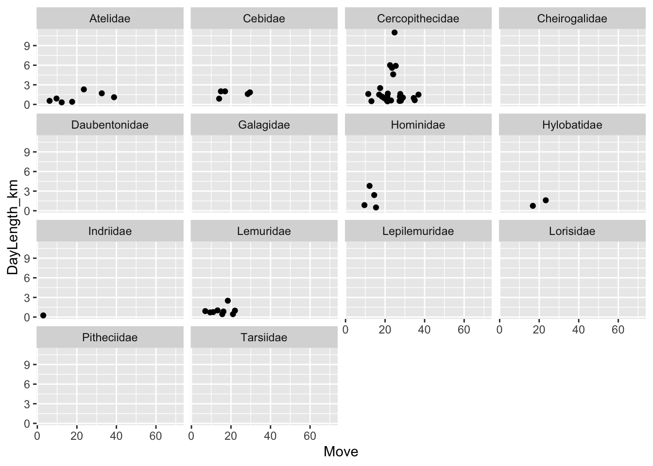
(p <- ggplot(data = d, aes(x = Move, y = DayLength_km)) +
  geom_point(na.rm = TRUE) +
  facet_wrap(~Family))

# 5
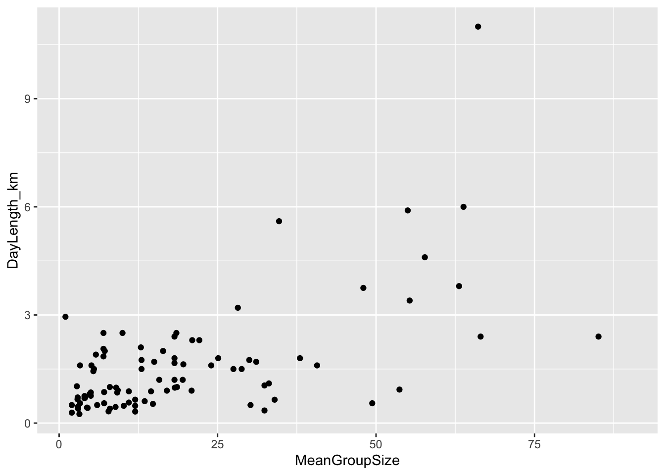
(p <- ggplot(data = d, aes(x = MeanGroupSize, y = DayLength_km)) +
  geom_point(na.rm = TRUE))

(p <- ggplot(data = d, aes(x = MeanGroupSize, y = DayLength_km)) +
  geom_point(na.rm = TRUE) +
  facet_wrap(~Family))

# 6
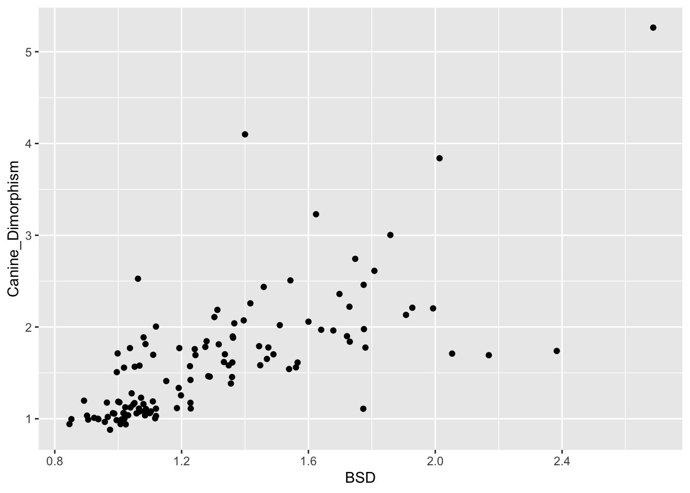
(p <- ggplot(data = d, aes(x = BSD, y = Canine_Dimorphism)) +
  geom_point(na.rm = TRUE))

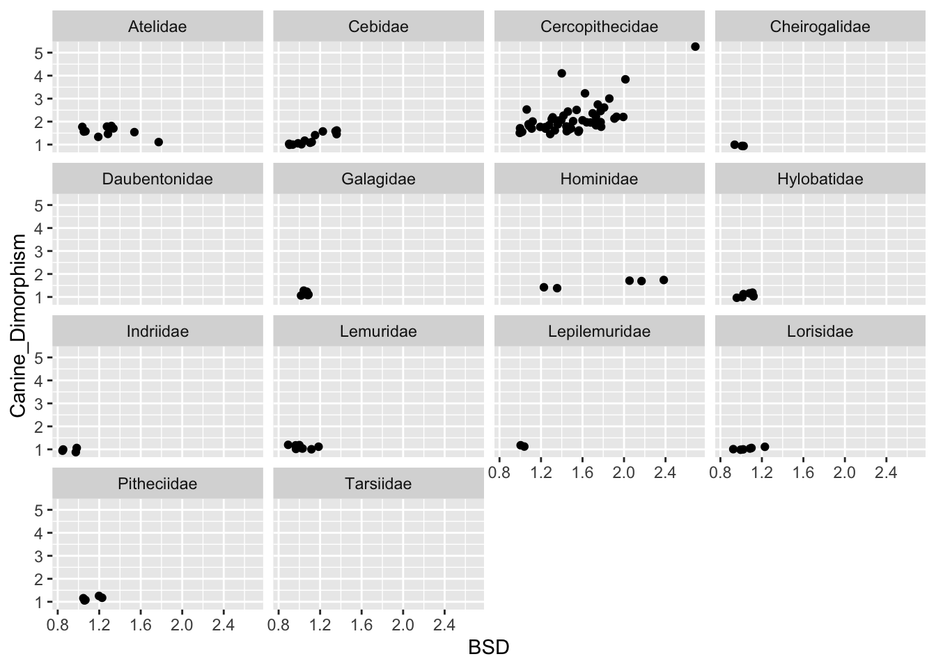
(p <- ggplot(data = d, aes(x = BSD, y = Canine_Dimorphism)) +
  geom_point(na.rm = TRUE)) +
  facet_wrap(~Family)

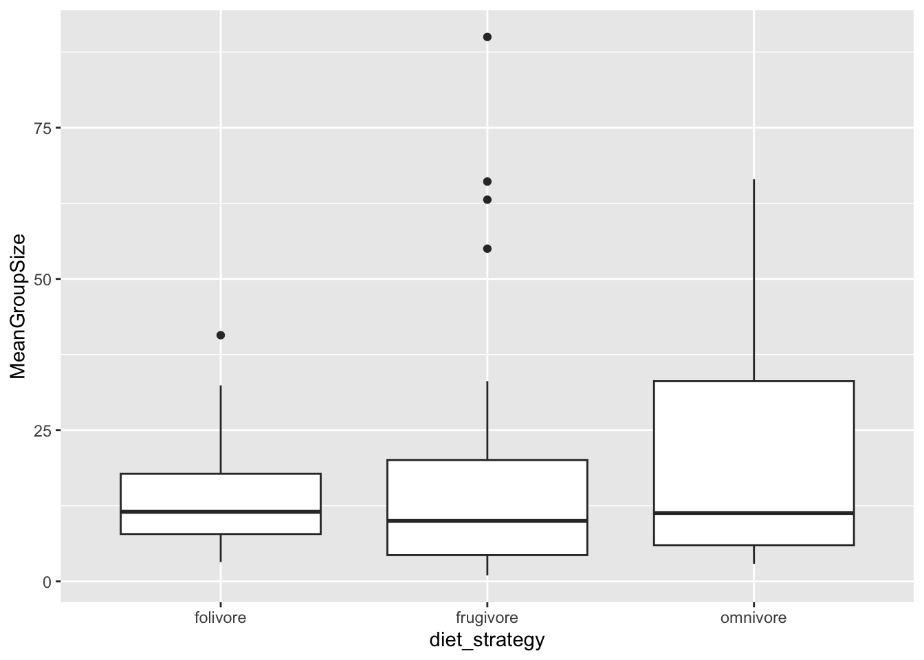
# 7
d <- d |> mutate(
  "diet_strategy" = case_when(
    Fruit >= 50 ~ "frugivore",
    Leaves >= 50 ~ "folivore",
    Fruit < 50 & Leaves < 50 ~ "omnivore",
    TRUE ~ NA
  )
)

(p <- ggplot(data = filter(d, !is.na(diet_strategy)), aes(x = diet_strategy, y = MeanGroupSize)) +
  geom_boxplot())

## Warning: Removed 19 rows containing non-finite outside the scale range
## (`stat_boxplot()`).

# 8
d <- d |>
  mutate(Binomial = paste0(Genus, " ", Species)) |>
  select(
    Binomial,
    Family,
    Brain_Size_Species_Mean,
    Body_mass_male_mean
  ) |>
  group_by(Family) |>
  summarise(
    meanBrainSize = mean(Brain_Size_Species_Mean, na.rm = TRUE),
    meanMaleBodySize = mean(Body_mass_male_mean, na.rm = TRUE)
  ) |>
  arrange(meanBrainSize) |>
  print()

## # A tibble: 14 × 3
##    Family          meanBrainSize meanMaleBodySize
##    <chr>                   <dbl>            <dbl>
##  1 Tarsiidae                3.26             131 
##  2 Cheirogalidae            4.04             193.
##  3 Galagidae                5.96             395.
##  4 Lepilemuridae            7.27             792 
##  5 Lorisidae                8.67             512.
##  6 Lemuridae               23.1             2077.
##  7 Cebidae                 23.9             1012.
##  8 Indriidae               27.3             3638.
##  9 Daubentonidae           44.8             2620 
## 10 Pitheciidae             56.3             1955.
## 11 Atelidae                80.6             7895.
## 12 Cercopithecidae         85.4             9543.
## 13 Hylobatidae            101.              6926.
## 14 Hominidae              410.             98681.