Exercise 08 Solution

• Solution

Challenge

Step 1

Using the {tidyverse} read_csv() function, load the “Street_et_al_2017.csv” dataset as a “tibble” named d.

library(tidyverse)
library(broom)
f <- "https://raw.githubusercontent.com/difiore/ada-datasets/main/Street_et_al_2017.csv"
d <- read_csv(f, col_names = TRUE)

Do a quick exploratory data analysis where you generate the five-number summary (median, minimum and maximum and 1st and 3rd quartile values), plus mean and standard deviation, for each quantitative variable.

library(skimr)
library(kableExtra)
skim(d) |>
  kable() |>
  kable_styling(font_size = 10, full_width = FALSE)

skim_type	skim_variable	n_missing	complete_rate	character.min	character.max	character.empty	character.n_unique	character.whitespace	numeric.mean	numeric.sd	numeric.p0	numeric.p25	numeric.p50	numeric.p75	numeric.p100	numeric.hist
character	Species	0	1.0000000	10	41	0	301	0	NA	NA	NA	NA	NA	NA	NA	NA
character	Taxonomic_group	0	1.0000000	10	12	0	3	0	NA	NA	NA	NA	NA	NA	NA	NA
numeric	Social_learning	98	0.6744186	NA	NA	NA	NA	NA	2.300493	16.51382	0.000	0.0000	0.000	0.0000	214.00	▇▁▁▁▁
numeric	Research_effort	115	0.6179402	NA	NA	NA	NA	NA	38.763441	80.58897	1.000	6.0000	16.000	37.7500	755.00	▇▁▁▁▁
numeric	ECV	117	0.6112957	NA	NA	NA	NA	NA	68.493206	82.84154	1.630	11.8250	58.550	86.1975	491.27	▇▁▁▁▁
numeric	Group_size	114	0.6212625	NA	NA	NA	NA	NA	13.263102	15.19637	1.000	3.1250	7.500	18.2250	91.20	▇▂▁▁▁
numeric	Gestation	161	0.4651163	NA	NA	NA	NA	NA	164.504000	37.99758	59.990	138.3525	166.030	183.2650	274.78	▁▅▇▃▁
numeric	Weaning	185	0.3853821	NA	NA	NA	NA	NA	311.088276	253.08157	40.000	121.6600	234.165	388.7825	1260.81	▇▃▁▁▁
numeric	Longevity	181	0.3986711	NA	NA	NA	NA	NA	331.971333	165.67434	103.000	216.0000	301.200	393.3000	1470.00	▇▂▁▁▁
numeric	Sex_maturity	194	0.3554817	NA	NA	NA	NA	NA	1480.228692	999.22681	283.180	701.5200	1427.170	1894.1100	5582.93	▇▆▂▁▁
numeric	Body_mass	63	0.7906977	NA	NA	NA	NA	NA	6795.184328	14229.82563	31.230	739.4425	3553.500	7465.0000	130000.00	▇▁▁▁▁
numeric	Maternal_investment	197	0.3455150	NA	NA	NA	NA	NA	478.640000	292.06808	99.990	255.8850	401.350	592.2175	1492.30	▇▅▂▁▁
numeric	Repro_lifespan	206	0.3156146	NA	NA	NA	NA	NA	9064.974702	4601.56798	2512.157	6126.2200	8325.890	10716.5950	39129.57	▇▃▁▁▁

detach(package:kableExtra)
detach(package:skimr)

Step 2

From this dataset, plot brain size (ECV) as a function of social group size (Group_size), longevity (Longevity), juvenile period length (Weaning), and reproductive lifespan (Repro_lifespan).

library(cowplot)
p1 <- ggplot(data = d, aes(x = Group_size, y = ECV)) +
  geom_point()
p2 <- ggplot(data = d, aes(x = Longevity, y = ECV)) +
  geom_point()
p3 <- ggplot(data = d, aes(x = Weaning, y = ECV)) +
  geom_point()
p4 <- ggplot(data = d, aes(x = Repro_lifespan, y = ECV)) +
  geom_point()
plot_grid(p1, p2, p3, p4, nrow = 2)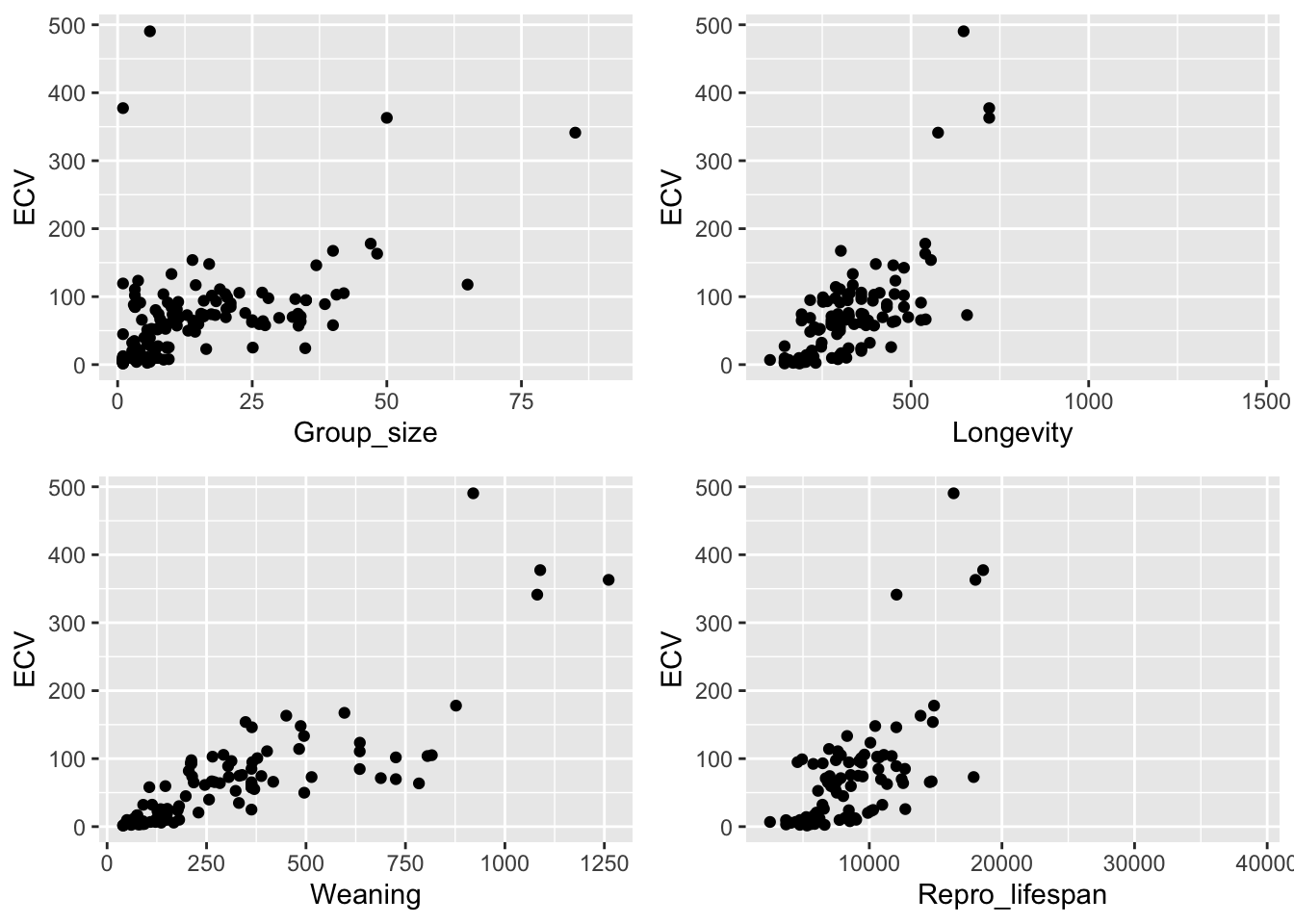

NOTE: It looks like most of these variables should probably be log transformed, though that is not essential for this exercise ;)

Step 3

Derive by hand the ordinary least squares regression coefficients \(\beta1\) and \(\beta0\) for ECV as a function of social group size.

d_mod <- d |> filter(!is.na(ECV) & !is.na(Group_size))
# or
d_mod <- d |> drop_na(ECV, Group_size)

(b1 <- cor(d_mod$ECV, d_mod$Group_size) * sd(d_mod$ECV) / sd(d_mod$Group_size))

## [1] 2.463071

(b0 <- mean(d_mod$ECV) - b1 * mean(d_mod$Group_size))

## [1] 30.35652

Step 4

Confirm that you get the same results using the lm() function.

m <- lm(ECV ~ Group_size, data = d_mod)
results <- m |>
  summary() |>
  tidy()
results

## # A tibble: 2 × 5
##   term        estimate std.error statistic  p.value
##   <chr>          <dbl>     <dbl>     <dbl>    <dbl>
## 1 (Intercept)    30.4      6.80       4.47 1.56e- 5
## 2 Group_size      2.46     0.351      7.02 7.26e-11

Step 5

Repeat the analysis above for three different major radiations of primates - “catarrhines”, “platyrrhines”, and “strepsirhines”) separately. Do your regression coefficients differ among groups? How might you determine this?

platyrrhini <- d_mod |> filter(Taxonomic_group == "Platyrrhini")
catarrhini <- d_mod |> filter(Taxonomic_group == "Catarrhini")
strepsirhini <- d_mod |> filter(Taxonomic_group == "Strepsirhini")

(platyrrhini_results <- lm(ECV ~ Group_size, data = platyrrhini) |>
  summary() |>
  tidy())

## # A tibble: 2 × 5
##   term        estimate std.error statistic  p.value
##   <chr>          <dbl>     <dbl>     <dbl>    <dbl>
## 1 (Intercept)    16.2      7.39       2.19 0.0356  
## 2 Group_size      1.97     0.455      4.32 0.000136

# or
(beta1_p <- cov(platyrrhini$ECV, platyrrhini$Group_size) / var(platyrrhini$Group_size))

## [1] 1.965176

(beta0_p <- mean(platyrrhini$ECV) - beta1_p * mean(platyrrhini$Group_size))

## [1] 16.18121

(catarrhini_results <- lm(ECV ~ Group_size, data = catarrhini) |>
  summary() |>
  tidy())

## # A tibble: 2 × 5
##   term        estimate std.error statistic     p.value
##   <chr>          <dbl>     <dbl>     <dbl>       <dbl>
## 1 (Intercept)    83.4     14.9        5.59 0.000000438
## 2 Group_size      1.15     0.579      1.98 0.0518

# or
(beta1_c <- cov(catarrhini$ECV, catarrhini$Group_size) / var(catarrhini$Group_size))

## [1] 1.146322

(beta0_c <- mean(catarrhini$ECV) - beta1_c * mean(catarrhini$Group_size))

## [1] 83.42059

(strepsirhini_results <- lm(ECV ~ Group_size, data = strepsirhini) |>
  summary() |>
  tidy())

## # A tibble: 2 × 5
##   term        estimate std.error statistic  p.value
##   <chr>          <dbl>     <dbl>     <dbl>    <dbl>
## 1 (Intercept)     8.18     2.14       3.83 0.000404
## 2 Group_size      1.84     0.473      3.89 0.000332

# or
(beta1_s <- cov(strepsirhini$ECV, strepsirhini$Group_size) / var(strepsirhini$Group_size))

## [1] 1.840664

(beta0_s <- mean(strepsirhini$ECV) - beta1_s * mean(strepsirhini$Group_size))

## [1] 8.176384

As seen from the results above, the coefficients do differ among groups… but how might we test if this difference is signficant? One way would be to permute the group assignments randomly, for each permutation, calculate the difference in slopes between pairs of groups to create permutation distributions for that test statistic under a null model of no difference between groups. We could then compare the observed difference in slopes between groups to the “expected” distribution under that specified null model.

Step 6

For your first regression of ECV on social group size, calculate the standard error for the slope coefficient, the 95% CI, and the p value associated with this coefficient by hand.

# first define alpha and degrees of freedom for the regression
alpha <- 0.05
p.lower <- alpha / 2
p.upper <- 1 - (alpha / 2)
n <- nrow(d_mod) # number of observations
df <- n - 2

# then, calculate residuals...
residuals <- d_mod$ECV - (b0 + b1 * d_mod$Group_size)
# or residuals <- m$residuals

# then, calculate the SE for b1...
SSE <- sum(residuals^2)
dfe <- nrow(d_mod) - 1 - 1 # number of observations - number of predictors - 1 = n - p - 1
MSE <- SSE / dfe
SSX <- sum((d_mod$Group_size - mean(d_mod$Group_size))^2)

(SE_b1 <- sqrt(MSE / SSX))

## [1] 0.3508061

# we can calculate an SE for b0 as well...
(SE_b0 <- SE_b1 * sqrt(sum(d_mod$Group_size^2) / n))

## [1] 6.796325

# calculated 95% CI for b1 assuming a t distribution...
(CI_b1 <- b1 + c(-1, 1) * qt(p = 1 - (alpha / 2), df = df) * SE_b1)

## [1] 1.769874 3.156269

# we can calculate a CI for b0 as well...
(CI_b0 <- b0 + c(-1, 1) * qt(p = 1 - (alpha / 2), df = df) * SE_b0)

## [1] 16.92690 43.78615

# calculate p values...
# first, we need t statistics...
t_b1 <- b1 / SE_b1
t_b0 <- b0 / SE_b0

(p_b1 <- pt(-1 * abs(t_b1), df = df, lower.tail = TRUE) + (1 - pt(abs(t_b1), df = df, lower.tail = TRUE)))

## [1] 7.259436e-11

# or
(p_b1 <- 2 * pt(abs(t_b1), df = df, lower.tail = FALSE))

## [1] 7.259435e-11

(p_b0 <- 2 * pt(abs(t_b0), df = df, lower.tail = FALSE))

## [1] 1.561214e-05

Also extract this same information from the results of running the lm() function. Compare the hand-calculated output above to that pulled from the model result object, m.

(results <- m |>
  summary() |>
  tidy(conf.int = TRUE, conf.level = 1 - alpha))

## # A tibble: 2 × 7
##   term        estimate std.error statistic  p.value conf.low conf.high
##   <chr>          <dbl>     <dbl>     <dbl>    <dbl>    <dbl>     <dbl>
## 1 (Intercept)    30.4      6.80       4.47 1.56e- 5    16.9      43.8 
## 2 Group_size      2.46     0.351      7.02 7.26e-11     1.77      3.16

Step 7

Then, use a permutation approach with 1000 permutations to generate a null sampling distribution for the slope coefficient.

library(mosaic)
library(infer)
# using a loop to get a permutation distribution for slope
nperm <- 1000
perm <- vector(length = nperm)
perm.sample <- d_mod
for (i in 1:nperm) {
  perm.sample$Group_size <- sample(perm.sample$Group_size)
  result <- lm(ECV ~ Group_size, data = perm.sample) |>
    tidy() |>
    filter(term == "Group_size") |>
    pull(estimate)
  perm[[i]] <- result
}
histogram(perm, xlim = c(-3, 3))

ladd(panel.abline(v = b1, lty = 3, lwd = 2))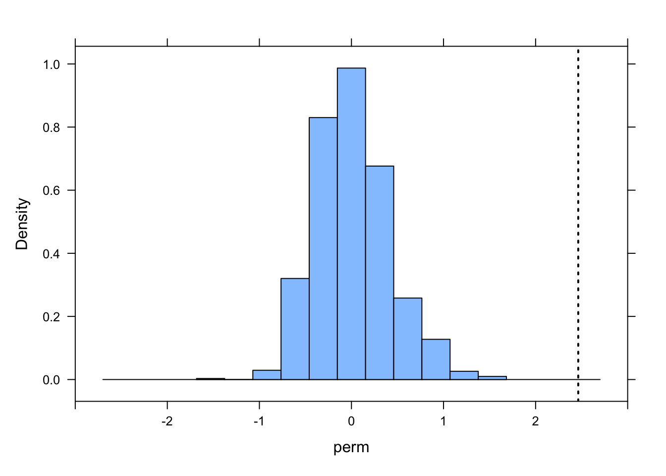

# calculate se as sd of permutation distribution
perm.se <- sd(perm)

# or, using the {infer} workflow...
perm <- d_mod |>
  # specify model
  specify(ECV ~ Group_size) |>
  # use a null hypothesis of independence
  hypothesize(null = "independence") |>
  # generate permutation replicates
  generate(reps = nperm, type = "permute") |>
  # calculate the slope statistic
  calculate(stat = "slope")

visualize(perm) + shade_p_value(obs_stat = b1, direction = "two_sided")

# calculate se as sd of permutation distribution
perm.se <- sd(perm$stat)

What is the p value associated with your original slope coefficient? You can use either the percentile method (i.e., using quantiles from actual permutation-based null sampling distribution) or a theory-based method (i.e., using the standard deviation of the permutation-based null sampling distribution as the estimate of the standard error), or both, to calculate this p value.

(p.percentile <- perm |>
  mutate(test = abs(stat) >= abs(b1)) |>
  summarize(p = mean(test)) |>
  pull(p))

## [1] 0

# p value taken directly from the permutation distribution i.e., how many of the slope estimates from permuted samples are more extreme than the actual b1?
# here, absolute value is used to make this a 2-tailed test

# or, using the {infer} package...
(p.percentile <- perm |> get_p_value(obs_stat = b1, direction = "two_sided"))

## Warning: Please be cautious in reporting a p-value of 0. This result is an approximation
## based on the number of `reps` chosen in the `generate()` step.
## ℹ See `get_p_value()` (`?infer::get_p_value()`) for more information.

## # A tibble: 1 × 1
##   p_value
##     <dbl>
## 1       0

(p.theory <- 2 * pt(abs(b1) / perm.se, df = df, lower.tail = FALSE))

## [1] 7.556287e-09

# the t statistic used in `pt()` to calculate the p values is `b1/se_b1`, where `se_b1` is estimated as the standard deviation of the permutation distribution (i.e., `1/perm_se`)
# the `2 *` the upper-tail probability in this calculation is to make this a 2-tailed test

Step 8

Use bootstrapping to generate a 95% CI for your estimate of the slope coefficient using both the quantile method and the theory-based method (i.e., based on the standard deviation of the bootstrapped sampling distribution). Do these CIs suggest that your slope coefficient is different from zero?

# using a loop to get a bootstrap distribution to generate a CI for the slope coefficient
nboot <- 1000
boot <- vector(length = nboot)
for (i in 1:nboot) {
  boot.sample <- sample_n(d_mod, nrow(d_mod), replace = TRUE)
  result <- lm(ECV ~ Group_size, data = boot.sample) |>
    tidy() |>
    filter(term == "Group_size") |>
    pull(estimate)
  boot[[i]] <- result
}
histogram(boot, xlim = c(b1 - 3, b1 + 3))

CI.quantile <- c(quantile(boot, p.lower), quantile(boot, p.upper))
ladd(panel.abline(v = CI.quantile, lty = 3, lwd = 2, col = "red"))

CI.theory <- b1 + c(-1, 1) * qt(p.upper, df = df) * sd(boot)
ladd(panel.abline(v = CI.theory, lty = 3, lwd = 2, col = "blue"))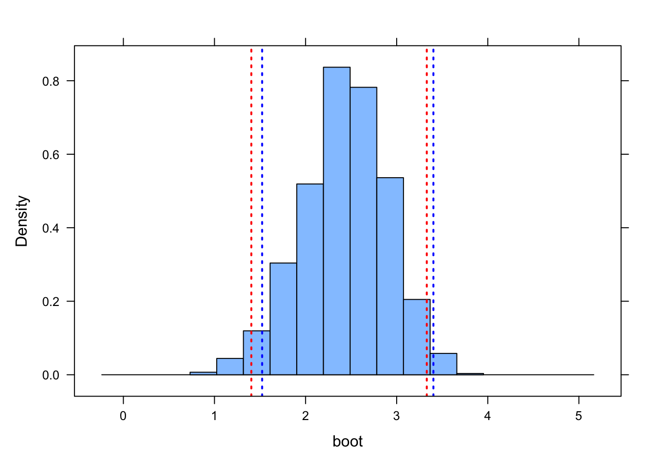

# or, using the {infer} workflow...
boot.slope <- d_mod |>
  # specify model
  specify(ECV ~ Group_size) |>
  # generate bootstrap replicates
  generate(reps = 1000, type = "bootstrap") |>
  # calculate the slope statistic
  calculate(stat = "slope")

(CI.quantile <- c(quantile(boot.slope$stat, p.lower), quantile(boot.slope$stat, p.upper)))

##     2.5%    97.5% 
## 1.512231 3.255595

# or...
(CI.quantile <- get_ci(boot.slope, level = 1 - alpha, type = "percentile", point_estimate = b1))

## # A tibble: 1 × 2
##   lower_ci upper_ci
##      <dbl>    <dbl>
## 1     1.51     3.26

(CI.theory <- b1 + c(-1, 1) * qt(p.upper, df = df) * sd(boot.slope$stat))

## [1] 1.565429 3.360713

# or...
(CI.theory <- get_ci(boot.slope, level = 1 - alpha, type = "se", point_estimate = b1))

## # A tibble: 1 × 2
##   lower_ci upper_ci
##      <dbl>    <dbl>
## 1     1.57     3.35

# note... the CI_theory values calculated with `get_ci()` differ very slightly from those calculated by hand because {infer} seems to be using upper/lower 0.025% boundaries of a *normal* rather than a *t* distribution
# I believe this is an "error" in how `get_ci()` is implemented in {infer}

visualize(boot.slope) +
  shade_ci(endpoints = CI.quantile, color = "red", fill = NULL) +
  shade_ci(endpoints = CI.theory, color = "blue", fill = NULL)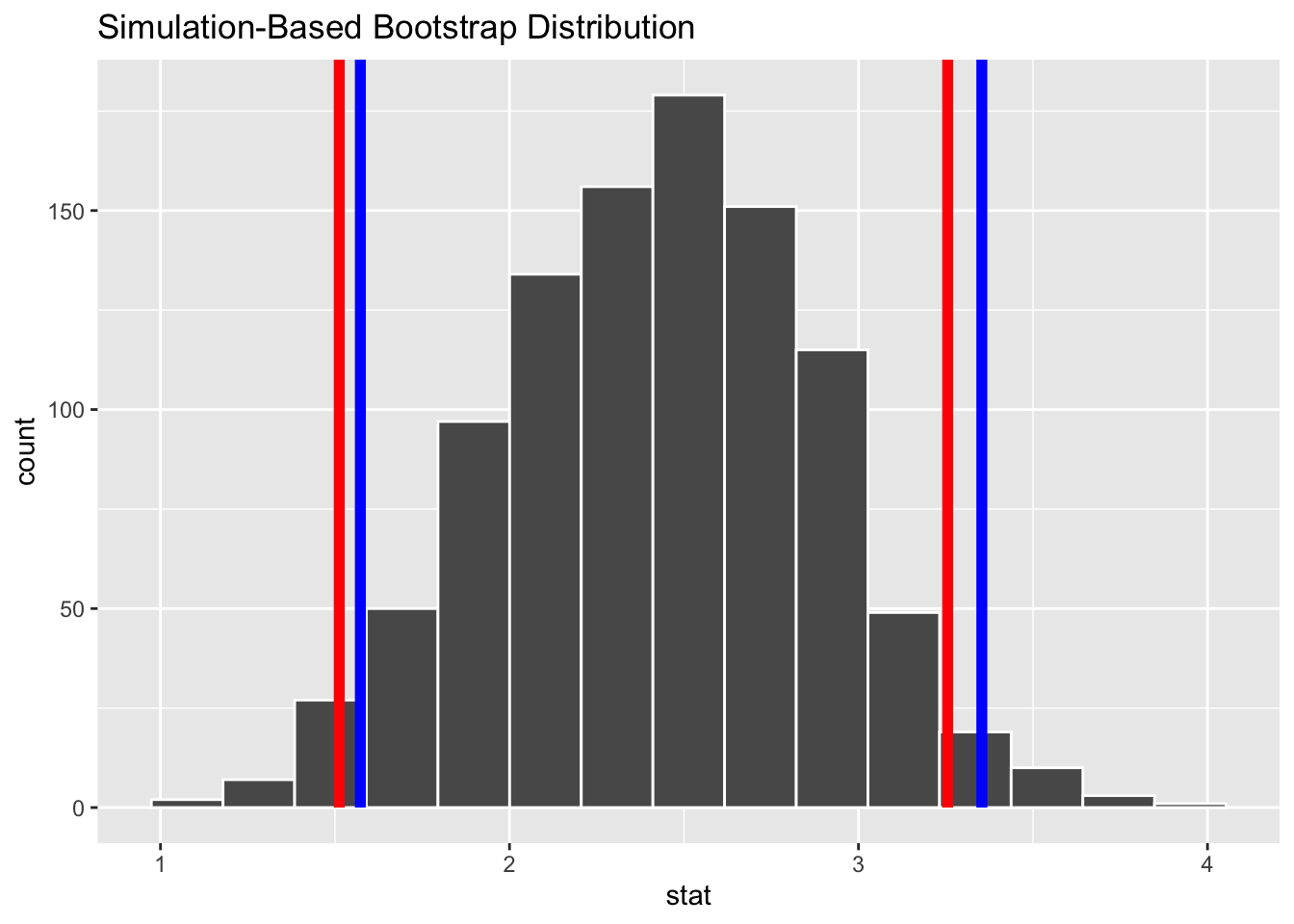

In all cases, none of these estimated CIs include zero, suggesting that the slope coefficient estimated in our linear model is “significant”.