4 Fundamentals of the R Language

4.1 Objectives

The goal of this module is to review important conceptual aspects of the R language as well as practices for updating R components of interest.

4.2 Preliminaries

Install this package in R: {renv}

4.3 R Objects

Almost everything in R can be thought of as an object, including variables, functions, complex data structures, and environments.

Classes, Modes, and Types

Objects in R fall into different classes. There are six basic (or atomic) classes that pertain to vector variables: numeric (real numbers), integer (integer numbers), character (for text), logical (Boolean values, i.e., TRUE or FALSE, represented as 1 and 0, respectively), complex (for imaginary numbers), raw (a rarely used type that stores data as raw bytes). An additional class, factor, is used for defined levels of categorical variables where, behind the scenes, factor levels are represented as integer numbers… we will talk more about factors later on). There are other classes beyond this set of basic ones that pertain to objects other than vectors. For example, tabular data structures have the have the class data.frame, and both built-in and user defined functions have the class function.

You can ask R to return the class of any object with the class() function, and R objects can have more than one class. You can think of class as being a property of an object that determines how generic functions operate with it.

Examples:

# class of a variable
x <- 4
class(x)

## [1] "numeric"

x <- "hi there"
class(x)

## [1] "character"

# class of a function
class(mean)

## [1] "function"

# class of a dataframe
d <- data.frame(v1 = c("a", "b"), v2 = c(1, 2), v3 = c(TRUE, FALSE))
class(d)

## [1] "data.frame"

In R, environments are objects as well.

What is the class of the global environment, where we have been binding values to variable names? To check, use class(globalenv()).

Show Code

class(globalenv())

Show Output

## [1] "environment"

Objects in R also each have a mode and a base type. These are often closely aligned with and similar or identical to the class of an object, but the three terms refer to slightly different things. If an object has no specific class assigned to it, its class is typically the same as its mode.

Mode is a mutually exclusive classification of objects, according to their basic structure. When we coerce an object to another basic structure, we are changing its mode but not necessarily the class.

# mode of a variable
x <- 4
mode(x)

## [1] "numeric"

x <- "hi there"
mode(x)

## [1] "character"

# mode of a function
mode(mean)

## [1] "function"

The typeof() a variable is often the same as its class and mode. The exception is for “factor” variables…

# type of a variable
x <- "male"
class(x)

## [1] "character"

typeof(x)

## [1] "character"

# coerce x to be a factor variable
x <- as.factor(x)
class(x)

## [1] "factor"

typeof(x)

## [1] "integer"

levels(x)

## [1] "male"

NOTE: For more details on the difference between the class, mode, and base type of an object, check out the book Advanced R, Second Edition by Hadley Wickham (RStudio).

Vectors

R also supports a variety of data structures for variable objects, the most fundamental of which is the vector. Vectors are variables consisting of one or more values of the same type, e.g., student’s grades on an exam. The class of a vector has to be one of the atomic data types described above. A scalar variable, such as a constant, is simply a vector with only one value.

There are lots of ways to create vectors… one of the most common is to use the c() or “combine” command:

x <- c(15, 16, 12, 3, 21, 45, 23)
x

## [1] 15 16 12  3 21 45 23

y <- c("once", "upon", "a", "time")
y

## [1] "once" "upon" "a"    "time"

z <- "once upon a time"
z

## [1] "once upon a time"

What is the class of the vector x? Of z? Use the class() function to check.

Show Code

class(x)

Show Output

## [1] "numeric"

Show Code

class(z)

Show Output

## [1] "character"

What happens if you try the following assignment: x <- c("2", 2, "zombies")? What is the class of vector x now?

Show Code

x <- c("2", 2, "zombies")
class(x)

Show Output

## [1] "character"

This last case is an example of coercion, which happens automatically and often behind the scenes in R. When you attempt to combine different types of elements in the same vector, they are coerced to all be of the same type – the most restrictive type that can accommodate all of the elements. This takes place in a fixed order: logical → integer → double → character. For example, combining a character and an integer yields a character; combining a logical and a double yields a double.

You can also deliberately coerce a vector to be represented as a different base type by using an as.*() function, like as.logical(), as.integer(), as.double(), as.character(), or as.factor().

x <- c(3, 4, 5, 6, 7)
x

## [1] 3 4 5 6 7

y <- as.character(x)
y

## [1] "3" "4" "5" "6" "7"

Another way to create vectors is to use the sequence operator, :, which creates a sequence of values from spanning from the left side of the operator to the right, in increments of 1:

x <- 1:10
x

##  [1]  1  2  3  4  5  6  7  8  9 10

x <- 10:1
x

##  [1] 10  9  8  7  6  5  4  3  2  1

x <- 1.3:10.5
x

##  [1]  1.3  2.3  3.3  4.3  5.3  6.3  7.3  8.3  9.3 10.3

NOTE: Wrapping an assignment in parentheses, as in the code block below, allows simultaneous assignment and printing to the console!

(x <- 40:45)

## [1] 40 41 42 43 44 45

We can also create more complex sequences using the seq() function, which takes several arguments:

x <- seq(from = 1, to = 10, by = 2)
# skips every other value
x

## [1] 1 3 5 7 9

x <- seq(from = 1, to = 10, length.out = 3)
# creates 3 evenly spaced values
x

## [1]  1.0  5.5 10.0

Attributes and Structure

Many objects in R also have attributes associated with them, which we can think of as metadata, or data describing the object. Some attributes are intrinsic to an object. For example, a useful attribute to know about a vector object is the number of elements in it, which can be queried using the length() function.

length(x)

## [1] 3

We can also get or assign arbitrary attributes to an object using the function attr(), which takes two arguments: the object whose attributes are being assigned and the name of the attribute.

# we can assign arbitary attributes to the vector x
attr(x, "date collected") <- "2019-01-22"
attr(x, "collected by") <- "Anthony Di Fiore"
attributes(x) # returns a list of attributes of x

## $`date collected`
## [1] "2019-01-22"
## 
## $`collected by`
## [1] "Anthony Di Fiore"

class(attributes(x)) # the class of a list is "list"

## [1] "list"

# a "list" is another R data structure
attr(x, "date collected") # returns the value of the attribute

## [1] "2019-01-22"

Finally, every object in R also has a structure, which can be queried using the str() command.

str(x) # structure of the variable x

##  num [1:3] 1 5.5 10
##  - attr(*, "date collected")= chr "2019-01-22"
##  - attr(*, "collected by")= chr "Anthony Di Fiore"

str(mean) # struture of the function mean

## function (x, ...)

str(globalenv()) # structure of the global environment

## <environment: R_GlobalEnv>

str(attributes(x)) # attribute names are stored as a list

## List of 2
##  $ date collected: chr "2019-01-22"
##  $ collected by  : chr "Anthony Di Fiore"

NOTE: The glimpse() function from the {dplyr} package also yields information on the structure of an object, sometimes in a more easily-readable format than str().

CHALLENGE:

Try some vector math using the console in RStudio:

Assign a sequence of numbers from 15 to 28 to a vector, x.

NOTE: There are at least two different ways to do this!

Then, assign a sequence of numbers from 1 to 4 to a vector, y.
Finally, add x and y. What happens?

Show Code

x <- 15:28 # or x <- c(15, 16, 17...)
y <- 1:4
(x + y)

Show Output

##  [1] 16 18 20 22 20 22 24 26 24 26 28 30 28 30

Use the up arrow to recall the last command from history and modify the command to store the result of the addition to a variable, z. What kind of object is z? Examine it using the class() function. What is the length of z?

Now, think carefully about this output… there are two important things going on.

First, R has used vectorized addition in creating the new variable. The first element of x was added to the first element of y, the second element of x was added to the second element of y, etc.

Second, in performing this new variable assignment, the shorter vector has been recycled. Thus, once we get to the fifth element in x we start over with the first element in y.

This means we can very easily do things like adding a constant to all of the elements in a vector or multiplying all the elements by a constant.

y <- 2
# note that we can wrap a command in parentheses for simultaneous assignment/operation and printing
(z <- x + y)

##  [1] 17 18 19 20 21 22 23 24 25 26 27 28 29 30

(z <- x * y)

##  [1] 30 32 34 36 38 40 42 44 46 48 50 52 54 56

Many function operations in R are also vectorized, meaning that if argument of a function is a vector, but the function acts on a single value, then the function will be applied to each value in the vector and will return a vector of the same length where the function has been applied to each element.

x <- 1:20
(logx <- log(x))

##  [1] 0.0000000 0.6931472 1.0986123 1.3862944 1.6094379 1.7917595 1.9459101
##  [8] 2.0794415 2.1972246 2.3025851 2.3978953 2.4849066 2.5649494 2.6390573
## [15] 2.7080502 2.7725887 2.8332133 2.8903718 2.9444390 2.9957323

(x2 <- x^2)

##  [1]   1   4   9  16  25  36  49  64  81 100 121 144 169 196 225 256 289 324 361
## [20] 400

(y <- 4 * x + 3)

##  [1]  7 11 15 19 23 27 31 35 39 43 47 51 55 59 63 67 71 75 79 83

We can use the {base} R function plot() to do some quick visualizations.

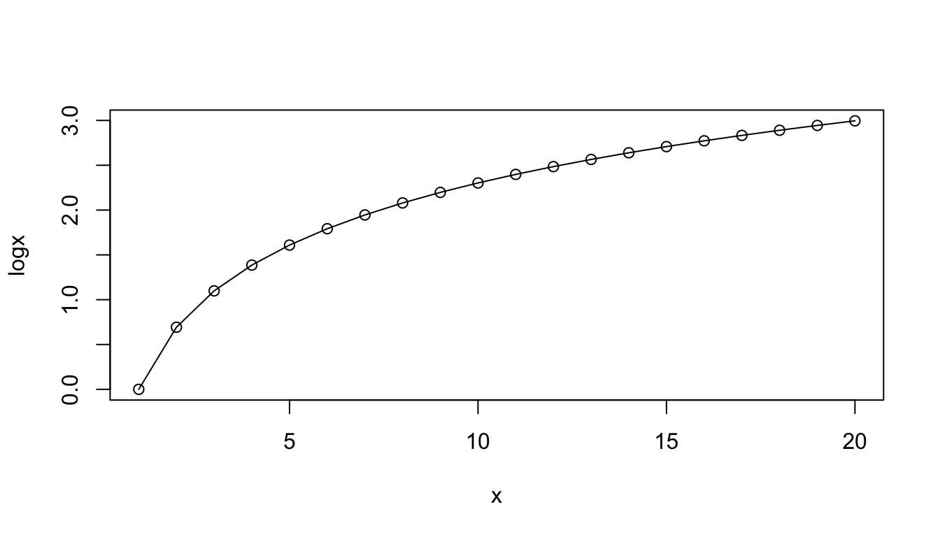
# `plot()` takes values of x and y values as the first two arguments, and the `type="o"` argument superimposes points and lines
plot(x, logx, type = "o")

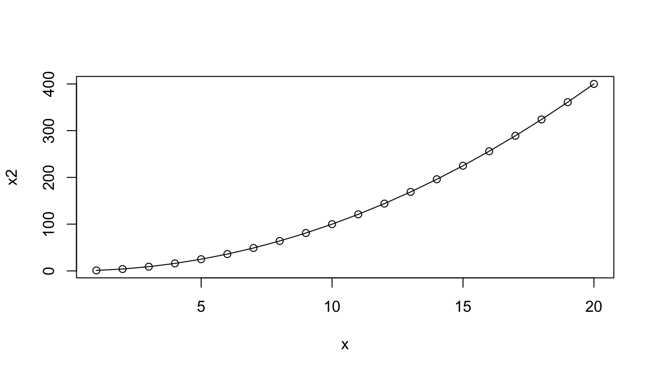
plot(x, x2, type = "o")

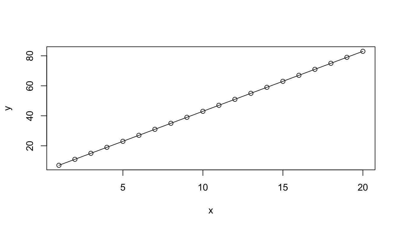
plot(x, y, type = "o")

CHALLENGE:

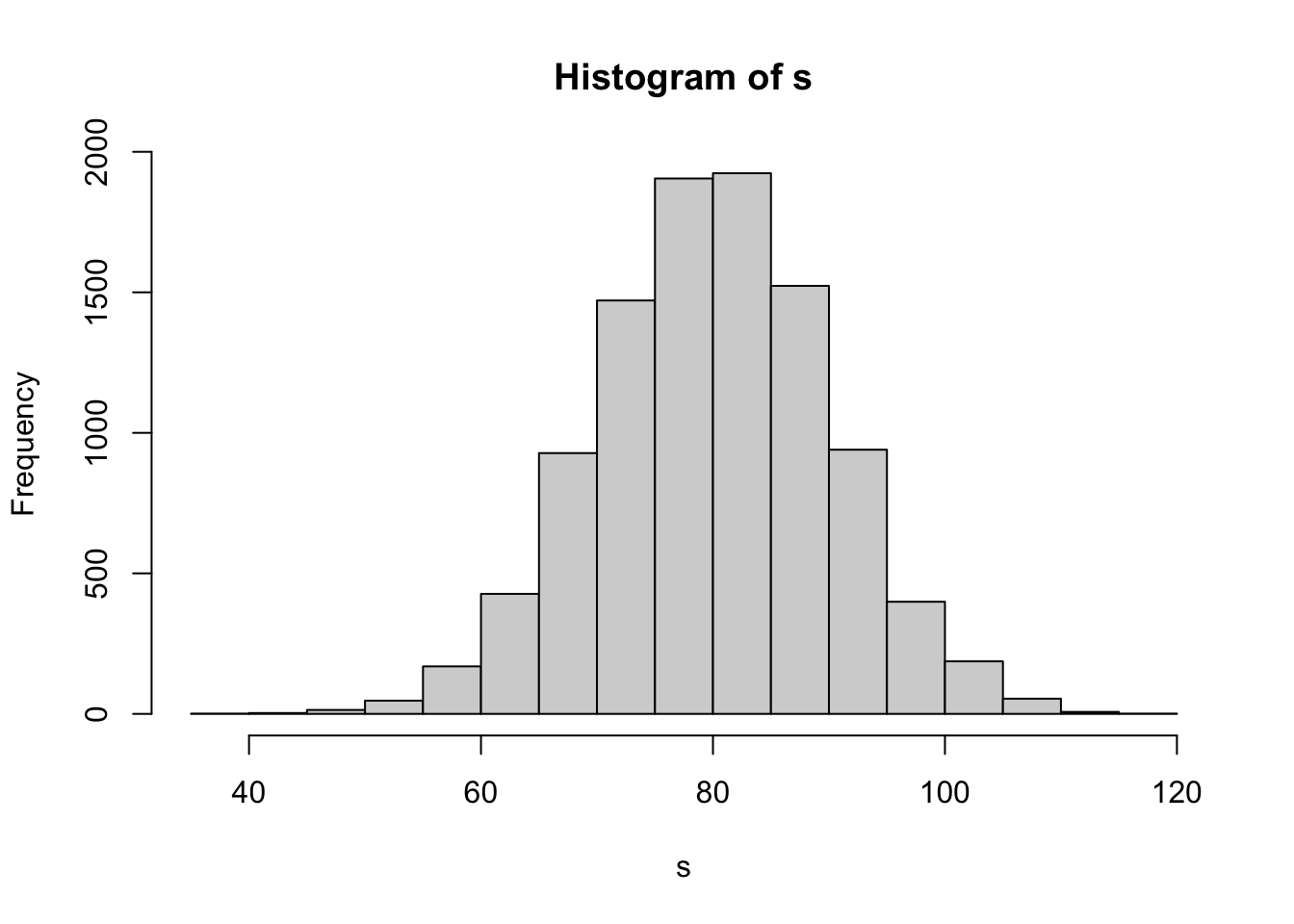
Use the rnorm() function to create a vector, s that contains a set of random numbers drawn from a normal distribution with mean 80 and standard deviation 10. Try doing this with n = 10, n = 100, n = 1000, n = 10000.

HINT: Use ?rnorm or help(rnorm) to access the help documentation on how to use the rnorm() function.

Then, use the hist() function to plot a histogram showing the distribution of these numbers.

Show Code

s <- rnorm(n = 10000, mean = 80, sd = 10)
hist(s) # hist() plots a simple histogram of values for s

Use the mean() and sd() functions to calculate the mean and standard deviation of s. Here, the whole vector is used as the argument of the function, i.e., the function applies to a set of values not a single value. The function thus returns a vector of length 1.

Show Code

mean(s)

Show Output

## [1] 80.04202

Show Code

sd(s)

Show Output

## [1] 10.02246

4.4 Scripts and Functions

As mentioned previously, scripts in R are simply text files that store an ordered list of commands, which can be used to link together sets of operations to perform complete analyses and show results.

For example, you could enter the lines below into a text editor and then save the script in a file named “my_script.R” in a folder called src/ inside your working directory.

x <- 1:10
s <- sum(x)
l <- length(x)
m <- s / l
print(m)

## [1] 5.5

If you save a script, you can then use the source() function (with the path to the script file of interest as an argument) at the console prompt (or in another script) to read and execute the entire contents of the script file. In RStudio you may also go to Code > Source to run an entire script, or you can run select lines from within a script by opening the script text file, highlighting the lines of interest, and sending those lines to the console using the “Run” button or the appropriate keyboard shortcut, ⌘-RETURN (Mac) or control-ENTER (PC).

source("src/my_script.R")

## [1] 5.5

# assuming the file was saved with the ".R" extension...

In an R script, you might use several lines of code to accomplish a single analysis, but if you want to be able to flexibly perform that analysis with different input, it is good practice to organize portions of your code within a script into user-defined functions. A function is a bit of code that performs a specific task. It may take arguments or not, and it may return nothing, a single value, or any R object (e.g., a vector or a list, which is another data structure will discuss later on). If care is taken to write functions that work under a wide range of circumstances, then they can be reused in many different places. Novel functions are the basis of the thousands of user-designed packages that are what make R so extensible and powerful.

CHALLENGE:

Try writing a function!

Open a new blank document in RStudio
- File > New > R Script
Type in the code below to create the say_hi() function, which adds a name to a greeting:

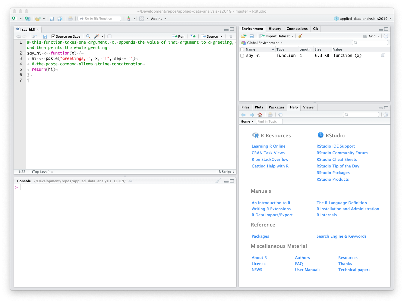
# this function takes one argument, `x`, appends the value of that argument to a greeting, and then prints the whole greeting
say_hi <- function(x) {
  hi <- paste("Greetings, ", x, "!", sep = "")
  return(hi)
}

NOTE: Here, the paste() command allows string concatenation. Alternatively, we could use the function paste0() and omit the sep= argument: hi <- paste0("Greetings, ", x, "!").

In general, the format for a function is as follows: function_name <- function(<arguments>) {<function code>}

You can send your new function to the R console by highlighting it in the editor and hitting ⌘-RETURN (Mac) or control-ENTER (PC). This loads the function as an object into the working environment.

Now we can create some test data and call the function. What are the results?

name1 <- "Rick Grimes"
name2 <- "Ruth Bader Ginsburg"
say_hi(name1)

## [1] "Greetings, Rick Grimes!"

say_hi(name2)

## [1] "Greetings, Ruth Bader Ginsburg!"

You can also save the function in a file and then run source("<path to file>") in code. Create an src/ folder inside your working directory, save your function script in that folder as “say_hi.R”, and then run the following:

source("src/say_hi.R")
name3 <- "Charles Darwin"
say_hi(name3)

## [1] "Greetings, Charles Darwin!"

4.5 Quitting R and Saving your Work

Working in RStudio, you can save script files (which, again, are just plain text files) using standard dialog boxes.

When you go to quit R (by using the q() function or by trying to close RStudio), you may be asked whether you want to…

“Save workspace image to <path>/.Rdata?”, where <path> is the path to your working directory.

Saying “Save” will store all of the contents of your workspace in a single hidden file, named “.Rdata”, inside of the working directory. The leading period (“.”) makes this invisible to most operating systems, unless you deliberately make it possible to see hidden files.

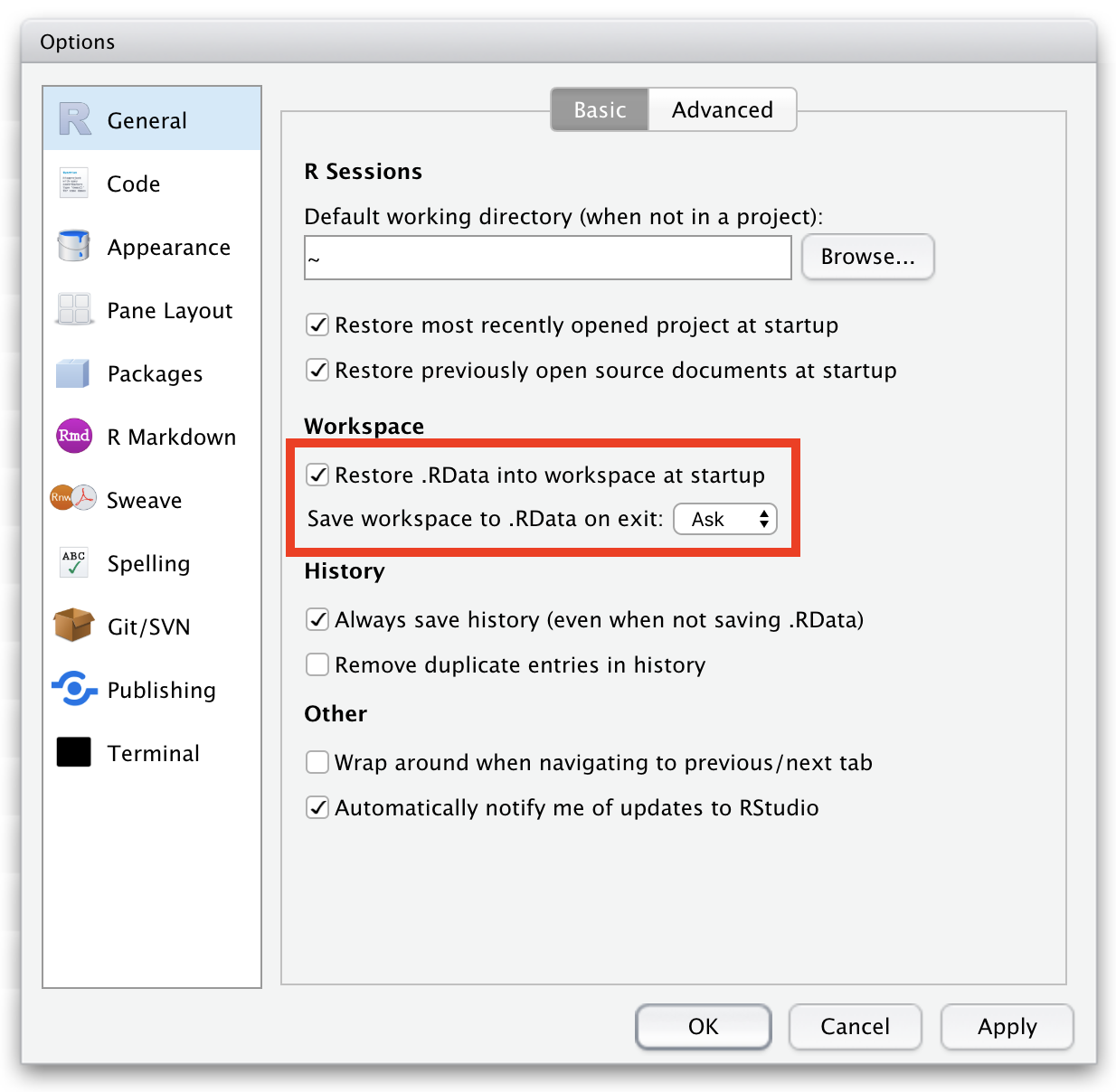
NOTE: I tend to NOT save my workspace images. You can change the default behavior for this by editing RStudio’s preferences. To do so, go to Tools > Global Options, select the “General” tab, and then choose “Always”, “Never”, or “Ask” under “Save workspace to .RData on exit”.

The next time you start R, the workspace from “.RData” will be loaded again automatically, provided you have not changed your working directory and you have not unchecked “Restore .RData into workspace at startup” in preferences.

A second hidden file, “.Rhistory”, will also be stored in the same directory, which will contain a log of all commands you sent to the console, provided you have not unchecked “Always save history”. You can clear your history in the RStudio IDE by clicking the broom icon on the History tab.

4.6 Updating R

R has been under continuous and active development since its inception in the late 1990s, and, typically, multiple updates are made available each year. These updates help to fix bugs, improve speed and computational efficiency, and add new functionality to the software. The following information on how to update R is based on this post from Stack Overflow

Step 1: Get the latest version of R
- Go to the R Project website.
- Click on CRAN in the sidebar on the left.
- Choose the CRAN Mirror site that you like.
- Click on Download R for… (choose your operating system).
- Follow the installation procedures for your system.
- Restart RStudio.
Step 2: Relocate your packages
- To ensure that your packages work with your new version of R, you need to:
  - Move the packages from your old R installation into the new one.
  - On MacOS, this typically means moving all library folders from either… “/Users/<username>/Library/R/<architecture>/<old-R-version>/library” to “/Users/<username>/Library/R/<architecture>/<new-R-version>/library” (for packages installed to a user library) or from… “/Library/Frameworks/R.framework/Versions/<old R-version>/Resources/library” to “/Library/Frameworks/R.framework/Versions/<new R-version>/Resources/library” (for packages installed to the system library)

NOTE: You will need to replace <username>, <architecture>, <old R-version>, and <new R-version> with your own user name, computer processor type, and versions of R you are upgrading from and to, respectively.

On Windows, this typically means moving all library folders from “C:\Program Files\R\<old R-version>\library” to “C:\Program Files\R\<new R-version>\library” (if your packages are installed at the system level) or from “C:\Users\\<username\>\R\win-library\<old R-version>\” to “C:\Users\<username\>\R\win-library\<new R-version>\” (if your packages are installed at the user level)

NOTE: You only need to copy whatever packages are not already in the destination directory, i.e., you do not need to overwrite your new {base} package, etc., with your old one.

If those paths do not work for you, try using installed.packages() or .libPaths() to find the proper path names. These may vary on your system, depending on where you installed R
Once you have moved your library folders, you should now can update all your packages by typing update.packages() in your RStudio console and answering “y” to all of the prompts or by going to the Packages tab, pressing the “Update” button, and then “Select All” and “Install Updates” to refresh all of your installed packages.
Finally, to reassure yourself that you have done everything correctly, type these two commands in the RStudio console to see what you’ve got in terms of what version of R you are running, the number of packages you have installed, and what packages you have loaded:

version # shows R version
packageStatus() # shows number of installed packages
(.packages()) # shows which packages are loaded

If you want to save a dataframe of all your installed packages, you can run…

my_packages <- as.data.frame(installed.packages())
write.csv(my_packages, "~/Desktop/my_packages.csv")

Often, packages build for an earlier version of R will work fine following an upgrade to a new version, but sometimes they do not. In that case, you can use the rebuild() function from the {renv} package to recompile each of your packages (and, by default, their dependencies)

library(renv)
rebuild(packages = my_packages$Package)

NOTE: With lots of installed packages, this can take some time! You can specify, instead, a single package or a shorter vector of packages using the packages = argument.

Concept Review

Characteristics of R objects: class(), mode(), typeof(), str(), attributes(), dplyr::glimpse()
Using scripts: source()
“.RData” and “.Rhistory” files
Updating R and installed packages

# Fundamentals of the ***R*** Language {#module-04} ## Objectives > The goal of this module is to review important conceptual aspects of the ***R*** language as well as practices for updating ***R*** components of interest. ## Preliminaries - Install this package in ***R***: [{renv}](https://cran.r-project.org/web/packages/easypackages/renv.pdf) ## ***R*** Objects Almost everything in ***R*** can be thought of as an *object*, including variables, functions, complex data structures, and environments. ### Classes, Modes, and Types {.unnumbered} Objects in ***R*** fall into different *classes*. There are six basic (or *atomic*) classes that pertain to vector variables: **numeric** (real numbers), **integer** (integer numbers), **character** (for text), **logical** (Boolean values, i.e., **TRUE** or **FALSE**, represented as 1 and 0, respectively), **complex** (for imaginary numbers), **raw** (a rarely used type that stores data as raw bytes). An additional class, **factor**, is used for defined levels of categorical variables where, behind the scenes, factor levels are represented as **integer** numbers... we will talk more about factors later on). There are other classes beyond this set of basic ones that pertain to objects other than vectors. For example, tabular data structures have the have the class **data.frame**, and both built-in and user defined functions have the class **function**. You can ask ***R*** to return the class of any object with the `class()` function, and ***R*** objects can have more than one class. You can think of class as being a property of an object that determines how generic functions operate with it. Examples: ```{r} # class of a variable x <- 4 class(x) x <- "hi there" class(x) # class of a function class(mean) # class of a dataframe d <- data.frame(v1 = c("a","b"), v2 = c(1,2), v3 = c(TRUE, FALSE)) class(d) ``` In ***R***, *environments* are objects as well. - What is the class of the *global environment*, where we have been binding values to variable names? To check, use `class(globalenv())`. ```{r} #| code-fold: true #| code-summary: "Show Code" #| attr.output: '.details summary="Show Output"' class(globalenv()) ``` Objects in ***R*** also each have a *mode* and a *base type*. These are often closely aligned with and similar or identical to the *class* of an object, but the three terms refer to slightly different things. If an object has no specific class assigned to it, its class is typically the same as its mode. Mode is a mutually exclusive classification of objects, according to their basic structure. When we coerce an object to another basic structure, we are changing its mode but not necessarily the class. ```{r} # mode of a variable x <- 4 mode(x) x <- "hi there" mode(x) # mode of a function mode(mean) ``` The `typeof()` a variable is often the same as its class and mode. The exception is for "factor" variables... ```{r} # type of a variable x <- "male" class(x) typeof(x) # coerce x to be a factor variable x <- as.factor(x) class(x) typeof(x) levels(x) ``` > **NOTE:** For more details on the difference between the *class*, *mode*, and *base type* of an object, check out the book [*Advanced R, Second Edition*](https://adv-r.hadley.nz/) by Hadley Wickham (RStudio). ### Vectors {.unnumbered} ***R*** also supports a variety of *data structures* for variable objects, the most fundamental of which is the *vector*. Vectors are *variables consisting of one or more values of the same type*, e.g., student's grades on an exam. The *class* of a vector has to be one of the atomic data types described above. A *scalar* variable, such as a constant, is simply a vector with only one value. - There are lots of ways to create vectors... one of the most common is to use the `c()` or "combine" command: ```{r} x <- c(15, 16, 12, 3, 21, 45, 23) x y <- c("once", "upon", "a", "time") y z <- "once upon a time" z ``` - What is the *class* of the vector **x**? Of **z**? Use the `class()` function to check. ```{r} #| code-fold: true #| code-summary: "Show Code" #| attr.output: '.details summary="Show Output"' class(x) class(z) ``` - What happens if you try the following assignment: `x <- c("2", 2, "zombies")`? What is the class of vector **x** now? ```{r} #| code-fold: true #| code-summary: "Show Code" #| attr.output: '.details summary="Show Output"' x <- c("2", 2, "zombies") class(x) ``` This last case is an example of *coercion*, which happens automatically and often behind the scenes in ***R***. When you attempt to combine different types of elements in the same vector, they are coerced to all be of the same type -- the most restrictive type that can accommodate all of the elements. This takes place in a fixed order: logical → integer → double → character. For example, combining a character and an integer yields a character; combining a logical and a double yields a double. You can also deliberately coerce a vector to be represented as a different base type by using an `as.*()` function, like `as.logical()`, `as.integer()`, `as.double()`, `as.character()`, or `as.factor()`. ```{r} x <- c(3, 4, 5, 6, 7) x y <- as.character(x) y ``` Another way to create vectors is to use the sequence operator, `:`, which creates a sequence of values from spanning from the left side of the operator to the right, in increments of 1: ```{r} x <- 1:10 x x <- 10:1 x x <- 1.3:10.5 x ``` > **NOTE:** Wrapping an assignment in parentheses, as in the code block below, allows simultaneous assignment and printing to the console! ```{r} (x <- 40:45) ``` We can also create more complex sequences using the `seq()` function, which takes several arguments: ```{r} x <- seq(from = 1, to = 10, by = 2) # skips every other value x x <- seq(from = 1, to = 10, length.out = 3) # creates 3 evenly spaced values x ``` ### Attributes and Structure {.unnumbered} Many objects in ***R*** also have *attributes* associated with them, which we can think of as metadata, or data describing the object. Some attributes are intrinsic to an object. For example, a useful attribute to know about a *vector* object is the number of elements in it, which can be queried using the `length()` function. ```{r} length(x) ``` We can also get or assign arbitrary attributes to an object using the function `attr()`, which takes two arguments: the object whose attributes are being assigned and the name of the attribute. ```{r} # we can assign arbitary attributes to the vector x attr(x, "date collected") <- "2019-01-22" attr(x, "collected by") <- "Anthony Di Fiore" attributes(x) # returns a list of attributes of x class(attributes(x)) # the class of a list is "list" # a "list" is another R data structure attr(x, "date collected") # returns the value of the attribute ``` Finally, every object in ***R*** also has a *structure*, which can be queried using the `str()` command. ```{r} str(x) # structure of the variable x str(mean) # struture of the function mean str(globalenv()) # structure of the global environment str(attributes(x)) # attribute names are stored as a list ``` > **NOTE:** The `glimpse()` function from the {dplyr} package also yields information on the structure of an object, sometimes in a more easily-readable format than `str()`. ### CHALLENGE: {.unnumbered} Try some vector math using the console in ***RStudio***: - Assign a sequence of numbers from 15 to 28 to a vector, **x**. > **NOTE:** There are at least two different ways to do this! - Then, assign a sequence of numbers from 1 to 4 to a vector, **y**. - Finally, add **x** and **y**. What happens? ```{r} #| warning: false #| code-fold: true #| code-summary: "Show Code" #| attr.output: '.details summary="Show Output"' x <- 15:28 # or x <- c(15, 16, 17...) y <- 1:4 (x + y) ``` - Use the up arrow to recall the last command from history and modify the command to store the result of the addition to a variable, **z**. What kind of object is **z**? Examine it using the `class()` function. What is the length of **z**? Now, think carefully about this output... there are two important things going on. First, ***R*** has used *vectorized* addition in creating the new variable. The first element of **x** was added to the first element of **y**, the second element of **x** was added to the second element of **y**, etc. Second, in performing this new variable assignment, the shorter vector has been *recycled*. Thus, once we get to the fifth element in **x** we start over with the first element in **y**. This means we can very easily do things like adding a constant to all of the elements in a vector or multiplying all the elements by a constant. ```{r} y <- 2 # note that we can wrap a command in parentheses for simultaneous assignment/operation and printing (z <- x + y) (z <- x * y) ``` Many function operations in ***R*** are also vectorized, meaning that if argument of a function is a vector, but the function acts on a single value, then the function will be applied to each value in the vector and will return a vector of the same length where the function has been applied to each element. ```{r} x <- 1:20 (logx <- log(x)) (x2 <- x^2) (y <- 4 * x + 3) ``` We can use the {base} ***R*** function `plot()` to do some quick visualizations. ```{r} #| fig-height: 4 #| out-width: "80%" # `plot()` takes values of x and y values as the first two arguments, and the `type="o"` argument superimposes points and lines plot(x, logx, type = "o") plot(x, x2, type = "o") plot(x, y, type = "o") ``` ### CHALLENGE: {.unnumbered} - Use the `rnorm()` function to create a vector, **s** that contains a set of random numbers drawn from a normal distribution with mean 80 and standard deviation 10. Try doing this with n = 10, n = 100, n = 1000, n = 10000. > **HINT:** Use `?rnorm` or `help(rnorm)` to access the help documentation on how to use the `rnorm()` function. Then, use the `hist()` function to plot a histogram showing the distribution of these numbers. ```{r} #| code-fold: true #| code-summary: "Show Code" #| attr.output: '.details summary="Show Output"' #| fig-align: center #| out-width: "80%" s <- rnorm(n = 10000, mean = 80, sd = 10) hist(s) # hist() plots a simple histogram of values for s ``` - Use the `mean()` and `sd()` functions to calculate the mean and standard deviation of **s**. Here, the whole vector is used as the argument of the function, i.e., the function applies to a set of values not a single value. The function thus returns a vector of length 1. ```{r} #| code-fold: true #| code-summary: "Show Code" #| attr.output: '.details summary="Show Output"' mean(s) sd(s) ``` ## Scripts and Functions As mentioned previously, scripts in ***R*** are simply text files that store an ordered list of commands, which can be used to link together sets of operations to perform complete analyses and show results. For example, you could enter the lines below into a text editor and then save the script in a file named "my_script.R" in a folder called `src/` inside your working directory. ```{r} x <- 1:10 s <- sum(x) l <- length(x) m <- s / l print(m) ``` If you save a script, you can then use the `source()` function (with the path to the script file of interest as an argument) at the console prompt (or in another script) to read and execute the entire contents of the script file. In ***RStudio*** you may also go to **Code > Source** to run an entire script, or you can run select lines from within a script by opening the script text file, highlighting the lines of interest, and sending those lines to the console using the "Run" button or the appropriate keyboard shortcut, `⌘-RETURN` (Mac) or `control-ENTER` (PC). ```{r} source("src/my_script.R") # assuming the file was saved with the ".R" extension... ``` In an ***R*** script, you might use several lines of code to accomplish a single analysis, but if you want to be able to flexibly perform that analysis with different input, it is good practice to organize portions of your code within a script into user-defined *functions*. A function is a bit of code that performs a specific task. It may take arguments or not, and it may return nothing, a single value, or any ***R*** object (e.g., a vector or a list, which is another data structure will discuss later on). If care is taken to write functions that work under a wide range of circumstances, then they can be reused in many different places. Novel functions are the basis of the thousands of user-designed packages that are what make ***R*** so extensible and powerful. ### CHALLENGE: {.unnumbered} Try writing a function! - Open a new blank document in ***RStudio*** - **File > New > R Script** - Type in the code below to create the `say_hi()` function, which adds a name to a greeting: ```{r} # this function takes one argument, `x`, appends the value of that argument to a greeting, and then prints the whole greeting say_hi <- function(x) { hi <- paste("Greetings, ", x, "!", sep = "") return(hi) } ``` > **NOTE:** Here, the `paste()` command allows string concatenation. Alternatively, we could use the function `paste0()` and omit the `sep=` argument: `hi <- paste0("Greetings, ", x, "!")`. In general, the format for a function is as follows: `function_name <- function(<arguments>) {<function code>}` You can send your new function to the ***R*** console by highlighting it in the editor and hitting `⌘-RETURN` (Mac) or `control-ENTER` (PC). This loads the function as an object into the working environment. ```{r} #| echo: false #| out-width: "90%" knitr::include_graphics("img/say_hi.png") ``` - Now we can create some test data and call the function. What are the results? ```{r} name1 <- "Rick Grimes" name2 <- "Ruth Bader Ginsburg" say_hi(name1) say_hi(name2) ``` You can also save the function in a file and then run `source("<path to file>")` in code. Create an `src/` folder inside your working directory, save your function script in that folder as "say_hi.R", and then run the following: ```{r} source("src/say_hi.R") name3 <- "Charles Darwin" say_hi(name3) ``` ## Quitting ***R*** and Saving your Work Working in ***RStudio***, you can save script files (which, again, are just plain text files) using standard dialog boxes. When you go to quit ***R*** (by using the `q()` function or by trying to close ***RStudio***), you may be asked whether you want to... "Save workspace image to \<path\>/.Rdata?", where \<path\> is the path to your working directory. Saying "Save" will store all of the contents of your workspace in a single *hidden* file, named ".Rdata", inside of the working directory. The leading period (".") makes this invisible to most operating systems, unless you deliberately make it possible to see hidden files. > **NOTE:** I tend to NOT save my workspace images. You can change the default behavior for this by editing ***RStudio***'s preferences. To do so, go to **Tools > Global Options**, select the "General" tab, and then choose "Always", "Never", or "Ask" under "Save workspace to .RData on exit". ```{r} #| echo: false #| out-width: "60%" knitr::include_graphics("img/rdata-prefs.png") ``` The next time you start ***R***, the workspace from ".RData" will be loaded again automatically, provided you have not changed your working directory and you have not unchecked "Restore .RData into workspace at startup" in preferences. A second hidden file, ".Rhistory", will also be stored in the same directory, which will contain a log of all commands you sent to the console, provided you have not unchecked "Always save history". You can clear your history in the ***RStudio*** IDE by clicking the broom icon on the **History** tab. ## Updating ***R*** ***R*** has been under continuous and active development since its inception in the late 1990s, and, typically, multiple updates are made available each year. These updates help to fix bugs, improve speed and computational efficiency, and add new functionality to the software. The following information on how to update ***R*** is based on [**this post from Stack Overflow**](http://stackoverflow.com/questions/13656699/update-r-using-rstudio) - Step 1: Get the latest version of ***R*** - Go to the [**R Project**](http://www.r-project.org) website. - Click on **CRAN** in the sidebar on the left. - Choose the **CRAN Mirror** site that you like. - Click on **Download R for...** (choose your operating system). - Follow the installation procedures for your system. - Restart ***RStudio***. - Step 2: Relocate your packages - To ensure that your packages work with your new version of ***R***, you need to: - Move the packages from your old ***R*** installation into the new one. - On MacOS, this typically means moving all library folders from either... "/Users/\<username\>/Library/R/\<architecture\>/\<old-R-version\>/library" to "/Users/\<username\>/Library/R/\<architecture\>/\<new-R-version\>/library" (for packages installed to a *user* library) or from... "/Library/Frameworks/R.framework/Versions/\<old R-version\>/Resources/library" to "/Library/Frameworks/R.framework/Versions/\<new R-version\>/Resources/library" (for packages installed to the *system* library) > **NOTE:** You will need to replace `<username>`, `<architecture>`, `<old R-version>`, and `<new R-version>` with your own user name, computer processor type, and versions of ***R*** you are upgrading from and to, respectively. - On Windows, this typically means moving all library folders from "C:\\Program Files\\R\\\<old R-version\>\\library" to "C:\\Program Files\\R\\\<new R-version\>\\library" (if your packages are installed at the *system* level) or from "C:\\Users\\\\<username\\>\\R\\win-library\\\<old R-version\>\\" to "C:\\Users\\\<username\\>\\R\\win-library\\<new R-version\>\\" (if your packages are installed at the *user* level) > **NOTE:** You only need to copy whatever packages are not already in the destination directory, i.e., you do not need to overwrite your new {base} package, etc., with your old one. - If those paths do not work for you, try using `installed.packages()` or `.libPaths()` to find the proper path names. These may vary on your system, depending on where you installed ***R*** - Once you have moved your library folders, you should now can update all your packages by typing `update.packages()` in your ***RStudio*** console and answering "y" to all of the prompts or by going to the *Packages* tab, pressing the "Update" button, and then "Select All" and "Install Updates" to refresh all of your installed packages. - Finally, to reassure yourself that you have done everything correctly, type these two commands in the ***RStudio*** console to see what you've got in terms of what version of ***R*** you are running, the number of packages you have installed, and what packages you have loaded: ```{r} #| eval: false version # shows R version packageStatus() # shows number of installed packages (.packages()) # shows which packages are loaded ``` If you want to save a dataframe of all your installed packages, you can run... ```{r} #| eval: FALSE my_packages <- as.data.frame(installed.packages()) write.csv(my_packages, "~/Desktop/my_packages.csv") ``` Often, packages build for an earlier version of ***R*** will work fine following an upgrade to a new version, but sometimes they do not. In that case, you can use the `rebuild()` function from the {renv} package to recompile each of your packages (and, by default, their dependencies) ```{r} #| eval: false library(renv) rebuild(packages = my_packages$Package) ``` > **NOTE:** With lots of installed packages, this can take some time! You can specify, instead, a single package or a shorter vector of packages using the `packages =` argument. --- ## Concept Review {.unnumbered} - Characteristics of ***R*** objects: `class()`, `mode()`, `typeof()`, `str()`, `attributes()`, `dplyr::glimpse()` - Using scripts: `source()` - ".RData" and ".Rhistory" files - Updating ***R*** and installed packages